
Click here to go to the corresponding page for the latest version of DIALS
Scaling of Beta-Lactamase dataset
Overview
Once the reflections have been integrated, a miller index, intensity and intensity error estimate have been determined for each measured reflection, in addition to information on the unit cell properties. However, before the data can be reduced for structure solution, the intensity values must be corrected for experimental effects which occur prior to the reflection being measured on the detector. These primarily include sample illumination/absorption effects and radiation damage, which result in symmetry-equivalent reflections having unequal measured intensities (i.e. a systematic effect in addition to any variance due to counting statistics). Thus the purpose of scaling is to determine a scale factor to apply to each reflection, such that the scaled intensities are representative of the ‘true’ scattering intensity from the contents of the unit cell.
Scaling is dependent on the space group symmetry assigned, which can be assessed
now that we have integrated intensities. Therefore first we shall run dials.symmetry
on the integrated.pickle and integrated_experiments.json files:
dials.symmetry integrated_experiments.json integrated.pickle
As can be seen from the output, the best solution is given by C 1 2/m 1,
in agreement with the result from dials.refine_bravais_settings.
To run scaling, any reflection files containing integrated reflections can be
passed to dials.scale. In the example below, we shall use the output files of
dials.symmetry, reindexed_experiments.json and
reindexed_reflections.pickle. When run, dials.scale performs scaling
on the dataset, and calculates an inverse scale factor for
each reflection (i.e. the corrected intensities are given by
\(I^{cor}_i = I^{obs}_i / g_i\)). The updated dataset is saved to
scaled.pickle, while details of the scaling model are saved in an
updated experiments file scaled_experiments.json. This can then be
used to produce an MTZ file for structure solution.
The scaling process
First, a scaling model must be created, from which we derive scale factors for
each reflection. By default, three components are used to create a physical model
for scaling (model=physical), in a similar manner to that used in the
program aimless. This model consists of a smoothly varying scale factor as a
function of rotation angle (scale_term), a smoothly varying B-factor to
account for radiation damage as a function of rotation angle (decay_term)
and an absorption surface correction, dependent on the direction of the incoming
and scattered beam vector relative to the crystal (absorption_term).
Let’s run dials.scale on the Beta-lactamase dataset, using a d_min cutoff:
dials.scale reindexed_experiments.json reindexed_reflections.pickle d_min=1.4
As can be seen from the log, a subset of reflections are selected to be used in scale factor determination, which helps to speed up the algorithm. In a typical rotation dataset, between 10 and 40 parameters will be used for each term of the model, therefore the problem is overdetermined and a subset of reflections can be used to determine the model components. Outlier rejection is performed at several stages, as outliers have a disproportionately large effect during scaling and can lead to poor scaling results.
Once the model has been initialised and a reflection subset chosen, the model parameters are be refined to give the best fit to the data, and then are used to calculate the scale factor for all reflections in the dataset. An error model is also optimised, to transform the intensity errors to an expected normal distribution. An error estimate for each scale factor is also determined based on the covariances of the model parameters. Finally, a table and summary of the merging statistics are presented, which give indications of the quality of the scaled dataset.
           ----------Overall merging statistics (non-anomalous)----------

Resolution: 69.19 - 1.40

Observations: 274776

Unique reflections: 41140

Redundancy: 6.7

Completeness: 94.11%

Mean intensity: 80.0

Mean I/sigma(I): 15.5

R-merge: 0.065

R-meas:  0.071

R-pim:   0.027
Inspecting the results
To see what the scaling is telling us about the dataset, plots of the scaling
model should be viewed. These can be generated by passing the output files to
the utility program dials.plot_scaling_models:
dials.plot_scaling_models scaled_experiments.json scaled.pickle
open scale_model.png absorption_surface.png
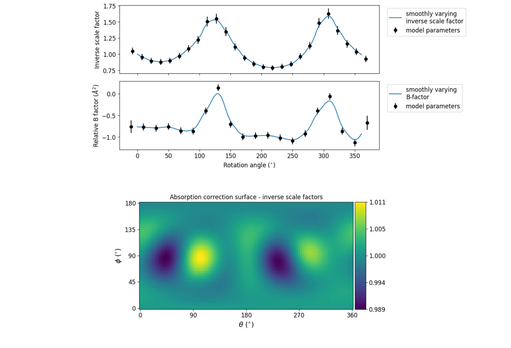
What is immediately apparent is the periodic nature of the scale term, with peaks
and troughs 90° apart. This indicates that the illumated volume was changing
significantly during the experiment: a reflection would be measured as twice as
intense if it was measured at rotation angle of ~120° compared to at ~210°.
The absorption surface also shows a similar periodicity, as may be expected.
What is less clear is the form of the relative B-factor, which also has a
periodic nature. As a B-factor can be understood to represent radiation damage,
this would not be expected to be periodic, and it is likely that this model
component is accounting for variation that could be described only by a scale
and absorption term. To test this, we can repeat the scaling process but turn
off the decay_term:
dials.scale reindexed_experiments.json reindexed_reflections.pickle d_min=1.4 decay_term=False
           ----------Overall merging statistics (non-anomalous)----------

Resolution: 69.19 - 1.40

Observations: 274585

Unique reflections: 41140

Redundancy: 6.7

Completeness: 94.11%

Mean intensity: 76.6

Mean I/sigma(I): 16.1

R-merge: 0.063

R-meas:  0.069

R-pim:   0.027
By inspecting the statistics in the output, we can see that removing the decay
term has had the effect of causing around 200 more reflections to be marked as
outliers (taking the outlier count from 0.75% to 0.82% of the data), while
improving some of the R-factors and mean I/sigma(I). Therefore it is probably
best to exclude the decay correction for this dataset.
Other options which could be explored are the numbers of parameters used for the
various components, for example by changing the scale_interval, or by
adjusting the outlier rejection criterion with a different outlier_zmax.
Exporting for further processing
Once we are happy with the results from scaling, the data can be exported as
an unmerged mtz file, for further symmetry analysis with pointless or to start
structural solution.
To obtain an unmerged mtz file, dials.export should be run, passing in
the output from scaling, with the option intensity=scale:
dials.export scaled.pickle scaled_experiments.json intensity=scale