
Click here to go to the corresponding page for the latest version of DIALS
Processing in Detail with DUI
Introduction
This tutorial follows the same steps as the command line tutorial Processing in Detail, but here processing will be driven graphically through the DIALS User Interface, DUI.
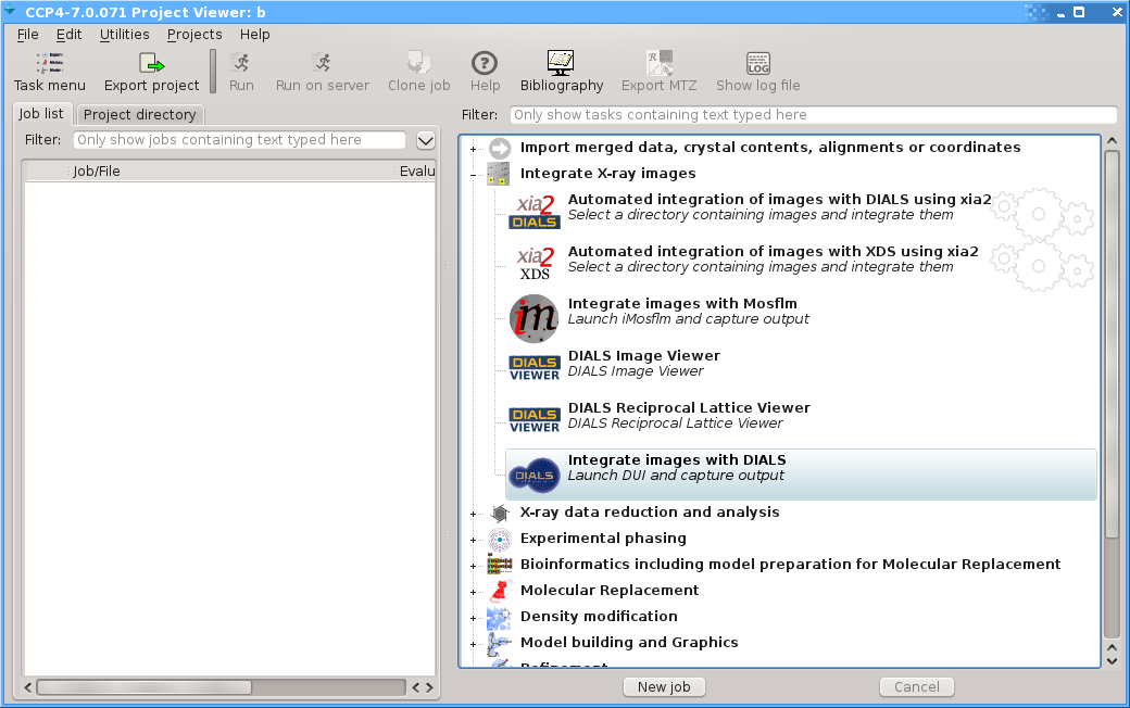
DUI is part of CCP4 and can be launched from ccp4i2 by selecting the relevant icon from within the “Integrate X-ray images” task folder.
Tutorial data
The following example uses a Beta-Lactamase dataset collected using beamline I04 at Diamond Light Source, and reprocessed especially for these tutorials.
Hint
If you are physically at Diamond on the CCP4 Workshop, then
this data is already available in your training data area. After
typing module load ccp4-workshop you’ll be moved to a working
folder, with the data already located in the tutorial-data/summed
subdirectory.
The data is otherwise available for download from ![]() .
We’ll only be using the first run of data in this tutorial,
.
We’ll only be using the first run of data in this tutorial,
C2sum_1.tar, extracted to a tutorial-data/summed subdirectory.
Import
When DUI starts up you will initially be presented by a window like the following.
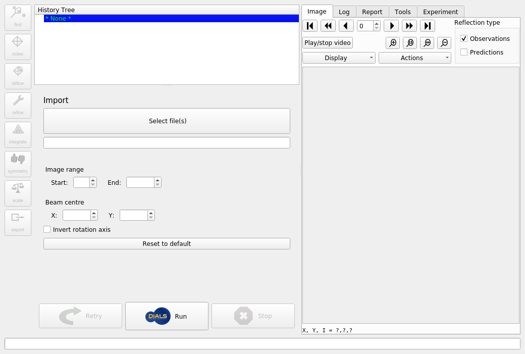
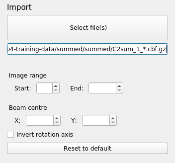
At this stage you can resize various parts of the interface until you are comfortable with the layout, but you can’t do much else until the dataset is imported by DIALS. To do this, click on the “Select File(s)” button, navigate to the location of the images and select any one of them. DUI will automatically determine the filename template and will show that with a wildcard in the text box. If there are problems with this template it is possible to edit this before importing the images. Otherwise, just click the “Run” button to proceed.
What happens then is that that the metadata are read for all the images in the dataset. If these are consistent, then the dataset is imported and initial models for the “Beam”, “Scan” and “Detector” are created. The images are now also displayed within the “Image” tab. You can adjust the contrast and colour scheme by controls under the “Display” pull-down.

Find Spots
The first “real” task in any processing using DIALS is the spot finding. To run this job, click on the “find” button at the upper-left of the window. When you do this you will see a new node will be created in the “History Tree”. This node is currently green, which indicates that it has not been run yet. By contrast, the import step is blue, which means this has been run. In general, it is always possible to navigate between each step of processing by clicking on the relevant position in the history. Advanced users will find this gives a great deal of control, allowing them to keep track of complex history, including parallel branches.
Spot-finding, like most of the other processing steps in DUI, presents user parameters at two levels of detail. The “Simple” tab contains the basic parameters that are the most commonly changed. The “Advanced” tab contains all of those again, plus other parameters that may be required for expert use with challenging data sets. In many cases, however, the default settings are fine.
Note that spot-finding is done on every image in the dataset. This means the job can take some time, but by default it will be run in parallel using multiple processors. To proceed, press the “Run” button below the input parameters.
Once the job is finished, the image viewer will display small blue boxes around the pixels that have been marked as strong. It is also useful to click on the “Report View” tab and scroll down to the “Analysis of strong reflections”. This shows a graph of the number of strong spots found per image. In this case there is a pretty steady rate of around 150 spots found on each image. If instead we had seen the number of strong spots drop off over the dataset, or otherwise show large variability we would start to worry about issues such as radiation damage or a poorly-centred crystal.
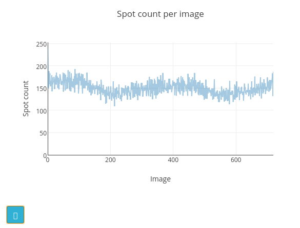
The cyan button at the bottom left of the graph opens a help window with a description of how the appearance of this plot may be affected by various data collection issues. In the “Log Text” window you can see the text output from the dials.find_spots program, which also includes an ASCII-art version of this plot.
The default parameters for spot finding usually do a good job for Pilatus images, such as these. However they may not be optimal for data from other detector types, such as CCDs or image plates. If you have a case where spot-finding has gone badly, it may be helpful to debug using the dials.image_viewer and dials.reciprocal_lattice_viewer, which can be launched via buttons shown on the “Tools” tab.
In particular, the effect of changing the spot-finding parameters can be explored interactively with the dials.image_viewer. The image mode buttons at the bottom of the “Settings” window allow a preview of how the parameters affect the spot finding algorithm. The final image, (“threshold”) is the one on which spots were found, so ensuring this produces peaks at real diffraction spot positions will give the best chance of success.
The second external viewer, the dials.reciprocal_lattice_viewer, displays the strong spots in 3D, after mapping them from their detector positions to reciprocal space. In a favourable case you should be able to see the crystal’s reciprocal lattice by eye in the strong spot positions. Some practice may be needed in rotating the lattice to an orientation that shows off the periodicity in reciprocal lattice positions.
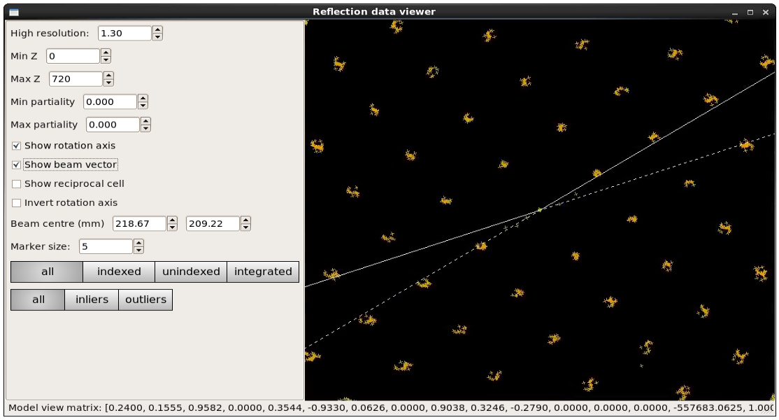
Although the reciprocal spacing is visible, in this data, there are clearly some systematic distortions. These will be solved during indexing.
Indexing
The next step will be indexing of the strong spots. Click on the “Index” button
to move on to this step, and form a new node in the history tree. Here we see
that the simple parameters allow only to select between different “Indexing
Methods”, the default of which is the 3D FFT algorithm. The other options are
the 1D FFT (DPS) algorithm and a special version of the 3D FFT called
real_space_grid_search, which is particularly useful for narrow wedges
containing multiple lattices, but requires a known cell and space group to be
set under the “Advanced” parameters. If we do know the cell and space group,
these can also be set as hints for either of the other two indexing algorithms.
This can help in difficult cases and will be used to constrain the lattice
during refinement. Otherwise
indexing and refinement will be carried out in the primitive lattice
using space group P1.
In this case, keep the method set to the default fft3d and click “Run” to
start the indexing job. Once the job has finished running, you can see in the
“Experiment” tab that the experimental models have now been completed with a
“Crystal” model.

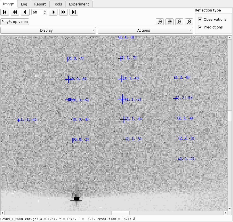
Now let’s click through the all the tabs of output. First, on the “Image” tab you will now see that indexed strong spots are assigned Miller indices. If you also click on the “Predictions” checkbox, under “Reflection Type” you will in addition see centroid positions and Miller indices for all predicted reflections, not just the strong spots.
Moving to the “Log Text” tab, it is worth reading through the output to understand what the indexing program has done. Inspecting the beginning of the log shows that the indexing step is done at a resolution lower than the full dataset; 1.84 Å:
Found max_cell: 94.4 Angstrom
Setting d_min: 1.84
FFT gridding: (256,256,256)
The resolution limit of data that can be used in indexing is determined by the size of the 3D FFT grid, and the likely maximum cell dimension. Here we used the default 256³ grid points. These are used to make an initial estimate for the unit cell parameters.
What then follows are ‘macro-cycles’ of refinement where the experimental model is first tuned to get the best possible fit from the data, and then the resolution limit is reduced to cover more data than the previous cycle. 16 parameters of the diffraction geometry are tuned: 6 for the detector, one for beam angle, 3 crystal orientation angles and the 6 triclinic cell parameters. At each stage only 36000 reflections are used in the refinement job. In order to save time, a subset of the input reflections are used - by default using 100 reflections for every degree of the 360° scan.
We see that the first macrocycle of refinement makes a big improvement in the positional RMSDs:
+--------+--------+----------+----------+------------+
|   Step |   Nref |   RMSD_X |   RMSD_Y |   RMSD_Phi |
|        |        |     (mm) |     (mm) |      (deg) |
|--------+--------+----------+----------+------------|
|      0 |  36000 | 0.56197  | 0.55131  |    0.13413 |
|      1 |  36000 | 0.24338  | 0.26503  |    0.15575 |
|      2 |  36000 | 0.10648  | 0.13198  |    0.13476 |
|      3 |  36000 | 0.055785 | 0.059567 |    0.10888 |
|      4 |  36000 | 0.051066 | 0.052336 |    0.10514 |
|      5 |  36000 | 0.050906 | 0.052372 |    0.10505 |
|      6 |  36000 | 0.050901 | 0.052378 |    0.10505 |
+--------+--------+----------+----------+------------+
Second and subsequent macrocycles are refined using the same number of reflections, but after extending to higher resolution. The RMSDs at the start of each cycle start off worse than at the end of the previous cycle, because the best fit model for lower resolution data is being applied to higher resolution reflections. As long as each macrocyle shows a reduction in RMSDs then refinement is doing its job of extending the applicability of the model out to a new resolution limit, until eventually the highest resolution strong spots have been included. The final macrocycle includes data out to 1.30 Å and produces a final model with RMSDs of 0.050 mm in X, 0.049 mm in Y and 0.104° in φ, corresponding to 0.29 pixels in X, 0.28 pixels in Y and 0.21 image widths in φ.
Despite the high quality of this data, we notice from the log that at each macrocycle there were some outliers identified and removed from refinement as resolution increases. Large outliers can dominate refinement using a least squares target, so it is important to be able to remove these. More about this is discussed below in Refinement. It’s also worth checking the total number of reflections that were unable to be assigned an index:
+------------+-------------+---------------+-------------+
|   Imageset |   # indexed |   # unindexed | % indexed   |
|------------+-------------+---------------+-------------|
|          0 |      107264 |           733 | 99.3%       |
+------------+-------------+---------------+-------------+
because this can be an indication of poor data quality or a sign that more care needs to be taken in selecting the indexing parameters.
Now the “Report View” contains more information than just after spot-finding. The “Spot count per image” plot also contains information about the number of indexed spots. In addition there are heat maps giving information about the positions of indexed and unindexed spots. Here we see that most of the unindexed spots are found in the region around the rotation axis. The “Analysis of reflection centroids” plots provide lots of detail regarding how well the predicted spot positions match the observed positions, both in image space and as a function of the position within the rotation scan.
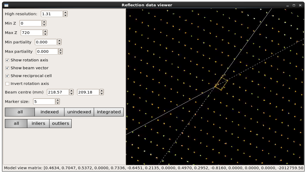
After indexing it can be useful to inspect the reciprocal lattice again under the “External Tools”. Now indexed/unindexed spots are differentiated by colour, and it is possible to see which spots were marked by dials.refine as outliers. If you have a dataset with multiple lattices present, it may be possible to spot them in the unindexed reflections.
In this case, we can see that the refinement has clearly resolved whatever systematic error was causing distortions in the reciprocal space view, and the determined reciprocal unit cell fits the data well:
Bravais Lattice Refinement
Since we didn’t know the Bravais lattice before indexing, we can now determine likely candidates - by taking the results of the P1 autoindexing, and running refinement with all of the possible Bravais settings applied. You can then choose your preferred solution. This step is accessed by the “Lattice” button on the left of the DUI window. As before, run this without altering any of the defaults, as they are suitable for the majority of data sets.
Once the job has run, a window will pop up containing scoring data and the unit cell for each Bravais setting.
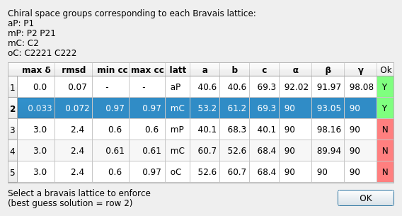
The scores for each setting include max δ (a metric fit measured in degrees), RMSDs (in mm), and the best and worse correlation coefficients for data related by symmetry elements (the symmetry elements implied by the lowest symmetry space group from the Bravais setting). This uses the raw spot intensity measurement from the spot-finding procedure (uncorrected and unscaled) but provides a very useful check to see if the data does appear to adhere to the proposed symmetry operators.
DIALS uses an heuristic to determine which solutions are acceptable or not, indicated on this window by either a green highlighted “Y” or a red highlighted “N”. In addition, the single “best” solution (the highest symmetry of the acceptable results) is pre-selected (highlighted in blue). To pick this solution, simply click “OK” while the chosen solution is highlighted. This will automatically apply the symmetry constraints and will reindex the reflections ready for further refinement.
Refinement
The model is already refined during indexing, but we can also add explicit refinement steps here. This is beneficial because it will use all reflections in refinement rather than a subset, uses a more sophisticated outlier rejection algorithm and will later allow us to fit a scan-varying model of the crystal.
We start by refining a static model including the monoclinic constraints from our chosen reindexed solution. For this we leave “Scan Varying Refinement” as “False”. There are various choices of outlier rejection algorithm allowed by refinement. The default selection of “auto” will choose the “mcd” algorithm for a rotation scan like this, which performs outlier rejection on the X, Y and φ residuals simultaneously, taking into account the multivariate nature of the data. This is appropriate for the ‘polishing up’ stage of refinement, whereas before during indexing the rougher, but less computationally expensive “tukey” option was used instead.
As before, click “Run” to start the job. The “Log Text” is familiar from the indexing stage. We see that all strong reflections were used in refinement, providing a small reduction in RMSDs. However, the refined model is still static over the whole dataset. We would like to do an additional refinement job at this point, to fit a more sophisticated model for the crystal, allowing small misset rotations to occur over the course of the scan. There are usually even small changes to the cell dimensions (typically resulting in a net increase in cell volume) caused by exposure to radiation during data collection. To account for both of these effects we can extend our parameterisation to obtain a smoothed scan-varying model for both the crystal orientation and unit cell.
This means running a further refinement job starting from the output of the previous job. To do that, note that the current “refine” node is a completed job and the parameters we entered are now greyed-out and cannot be edited. To do a second refinement starting from this point we simply click on the “refine” button again, opening a new green node in the history tree. Here we can select “Scan Varying Refinement” as “True” and click “Run” again to start the job.
The log output shows a decrease in each dimension, but especially in Y.
+--------+--------+----------+----------+------------+
|   Step |   Nref |   RMSD_X |   RMSD_Y |   RMSD_Phi |
|        |        |     (mm) |     (mm) |      (deg) |
|--------+--------+----------+----------+------------|
|      0 |  95415 | 0.045994 | 0.047882 |    0.1047  |
|      1 |  95415 | 0.043137 | 0.040683 |    0.10342 |
|      2 |  95415 | 0.041146 | 0.039717 |    0.1028  |
|      3 |  95415 | 0.040602 | 0.039511 |    0.10247 |
|      4 |  95415 | 0.040487 | 0.039501 |    0.10226 |
|      5 |  95415 | 0.040464 | 0.039497 |    0.10216 |
|      6 |  95415 | 0.040459 | 0.039496 |    0.10214 |
|      7 |  95415 | 0.040458 | 0.039497 |    0.10214 |
+--------+--------+----------+----------+------------+
The final RMSDs are less than a quarter of a pixel in both X and Y, and just under a fifth of a pixel in φ. This is about as good as we can expect from a high quality Pilatus data set such as this.
In the “Report View” we can now see plots of how the cell and orientation changes during the scan. The smoothness of these plots is guaranteed by the smoother model used by dials.refine. However, we are satisfied that this model is sufficient to match real changes present in the dataset because of the very low overall RMSDs.
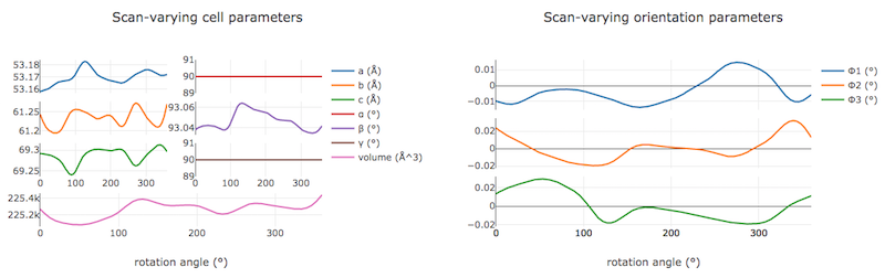
Other useful plots in the report are:
- Difference between observed and calculated centroids vs phi, which shows how the average residuals in each of X, Y, and φ vary as a fuction of φ. If scan-varying refinement has been successful in capturing the real changes during the scan then we would expect these plots to be straight lines.
- Centroid residuals in X and Y, in which the X, Y residuals are shown directly. The key point here is to look for a globular shape centred at the origin.
- Difference between observed and calculated centroids in X and Y, which show the difference between predicted and observed reflection positions in either X or Y as functions of detector position. From these plots it is very easy to see whole tiles that are worse than their neighbours, and whether those tiles might be simply shifted or slightly rotated compared to the model detector.
In this tutorial, we see no overall increase in all three cell parameters. If significant cell volume increases had been observed that might be indicative of radiation damage. However we can’t yet conclude that there is no radiation damage from the lack of considerable change observed.
Integration
After the refinement is done the next step is integration. Click on the “integrate” button to move to this job. Mostly, the default parameters are fine for Pilatus data, which will perform XDS-like 3D profile fitting while using a generalized linear model in order to fit a Poisson-distributed background model. As with spot-finding, the number of processes can be set >1 to speed the job up (but DUI will have selected a suitable default). Click “Run” to start integration. This is the most computationally-demanding stage of processing, so it will take a while to complete.
Checking the “Log Text” output, we see that after loading in the reference
reflections, new predictions are made up to the highest resolution at the
corner of the detector. This is fine, but if we wanted to we could have
adjusted the resolution limits using parameters d_min and d_max
under prediction in the “Advanced” parameters tab. The predictions are
made using the scan-varying crystal model from the previous step. As this
scan-varying model was determined in advance of integration, each of the
integration jobs is independent and we can take advantage of true parallelism
during processing.
The profile model is then calculated from the reflections file resulting from refinement. First reflections with a too small ‘zeta’ factor are filtered out. This essentially removes reflections that are too close to the spindle axis. In general these reflections require significant Lorentz corrections and as a result have less trustworthy intensities anyway. From the remaining reflection shoeboxes, the average beam divergence and reflecting range is calculated, providing the two Gaussian width parameters \(\sigma_D\) and \(\sigma_M\) used in the 3D profile model.
Following this, independent integration jobs are set up. These jobs overlap, so reflections are assigned to one or more jobs. What follows are blocks of information specific to each integration job.
After these jobs are finished, the reflections are ‘post-processed’, which includes the application of the LP correction to the intensities. Then summary tables are printed giving quality statistics first by frame, and then by resolution bin.
On the “Image View” tab we can now see integration “shoeboxes” around the spots, not just tight boxes around the strong pixels. If all stages up to this point have gone well, then the boxes should be centred on the strong pixels and should extend beyond the strong pixels to include pixels used for local background level determination.
The “Report View” now contains additional plots under the “Analysis of reflection intensities” and “Analysis of reference profiles” sections. It is worth checking through these, particularly paying attention to the following:
- Reflection and reference correlations binned in X/Y. These are useful companions to the plots of centroid residual as a function of detector position above. Whereas the above plots show systematic errors in the positions and orientations of tiles of a multi-panel detector, these plots indicate what effect that (and any other position-specific systematic error) has on the integrated data quality. The first of these plots shows the correlation between reflections and their reference profiles for all reflections in the dataset. The second shows only the correlations between the strong reference reflections and their profiles (thus these are expected to be higher and do not extend to such high resolution).
- Distribution of I/Sigma vs Z. This reproduces the \(\frac{I}{\sigma_I}\) information versus frame number given in the log file in a graphical form. Here we see that \(\frac{I}{\sigma_I}\) is fairly flat over the whole dataset, which we might use as an indication that there were no bad frames, not much radiation damage occurred and that scale factors are likely to be fairly uniform.
At this point we could export the integrated data set in MTZ format, however we will continue with this tutorial to demonstrate scaling within DIALS.
Checking the symmetry
After integration we can return to our hypothesis of the space group of the crystal. Although we made an assessment of that when we chose a Bravais lattice after indexing, we now have better, background-subtracted, values for the intensities, and for all reflections, not just the strong spots. So, it is prudent to repeat the assessment to see if there is any indication that our initial assessment should be revised.
This job is run using the “symmetry” button. We will again run with default settings only. Once the job is finished, check the “Log Text” output. The most important part here is the table printed at the end:
Scoring all possible sub-groups
---------------------------------------------------------------------------------------------
Patterson group       Likelihood  NetZcc  Zcc+   Zcc-   CC     CC-    delta  Reindex operator
---------------------------------------------------------------------------------------------
C 1 2/m 1        ***  0.909        9.72    9.72   0.00   0.97   0.00  0.0    -a,b,-c
P -1                  0.091        0.11    9.77   9.66   0.98   0.97  0.0    -x-y,-x+y,-z
---------------------------------------------------------------------------------------------
Best solution: C 1 2/m 1
Here we see clearly that the best solution is given by C 1 2/m 1, with
a high likelihood, in agreement with the result from
dials.refine_bravais_settings. As we remain confident with this choice,
we now continue to scaling.
Scaling
Before the data can be reduced for structure solution, the intensity values must be corrected for experimental effects which occur prior to the reflection being measured on the detector. These primarily include sample illumination/absorption effects and radiation damage, which result in symmetry-equivalent reflections having unequal measured intensities (i.e. a systematic effect in addition to any variance due to counting statistics). Thus the purpose of scaling is to determine a scale factor to apply to each reflection, such that the scaled intensities are representative of the ‘true’ scattering intensity from the contents of the unit cell.
During scaling, a scaling model is created, from which we derive scale factors for
each reflection. By default, three components are used to create a physical model
for scaling (model=physical), in a similar manner to that used in the
program aimless. This model consists of a smoothly varying scale factor as a
function of rotation angle, a smoothly varying B-factor to
account for radiation damage as a function of rotation angle
and an absorption surface correction, dependent on the direction of the incoming
and scattered beam vector relative to the crystal.
Let’s scale the Beta-lactamase dataset, after setting a resolution cutoff (d_min) of 1.4. This job is created by clicking the “scale” button. Enter 1.4 in the d_min field in the “simple” tab and click “Run” to start the job.
As can be seen from the “Log Text”, 70 parameters are used to parameterise the scaling model for this dataset. A subset of reflections are selected to be used in scaling model minimisation, which helps to speed up the algorithm (the model is used to calculate scales for all reflections at the end). Outlier rejection is performed at several stages, as outliers have a disproportionately large effect during scaling and can lead to poor scaling results. During scaling, the distribution of the intensity uncertainties are also analysed and an error model is optimised to transform the intensity errors to an expected normal distribution. An error estimate for each scale factor is also determined based on the covariances of the model parameters. At the end of the output, a table and summary of the merging statistics are presented, which give indications of the quality of the scaled dataset.
           ----------Overall merging statistics (non-anomalous)----------

Resolution: 69.19 - 1.40

Observations: 274799

Unique reflections: 41140

Redundancy: 6.7

Completeness: 94.11%

Mean intensity: 80.7

Mean I/sigma(I): 15.4

R-merge: 0.065

R-meas:  0.071

R-pim:   0.027
Inspecting the results
To see what the scaling is telling us about the dataset, plots of the scaling model should be viewed. These are visible within the “Report View” tab, at the bottom under “Analysis of scaling model”.
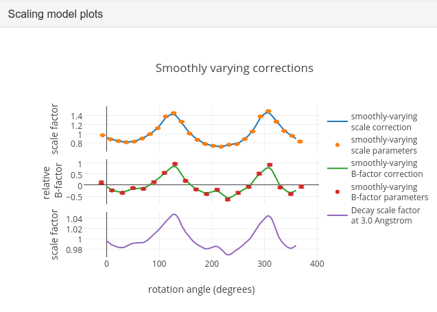
What is immediately apparent is the periodic nature of the scale term, with peaks
and troughs 90° apart. This indicates that the illuminated volume was changing
significantly during the experiment: a reflection would be measured as twice as
intense if it was measured at rotation angle of ~120° compared to at ~210°.
The absorption surface also shows a similar periodicity, as may be expected.
What is less clear is the form of the relative B-factor, which also has a
periodic nature. As a B-factor can be understood to represent radiation damage,
this would not be expected to be periodic, and it is likely that this model
component is accounting for variation that could be described only by a scale
and absorption term. To test this, we can repeat the scaling process but turn
off the decay_term.
To do this in DUI, click “Retry” to set up a new scaling job continuing from the successful symmetry-determination step. This time, enter the “Advanced” tab and under parameterisation change the value of decay_term to False. Now click “Run” to start the job.
           ----------Overall merging statistics (non-anomalous)----------

Resolution: 69.19 - 1.40

Observations: 274578

Unique reflections: 41140

Redundancy: 6.7

Completeness: 94.11%

Mean intensity: 76.6

Mean I/sigma(I): 16.0

R-merge: 0.064

R-meas:  0.070

R-pim:   0.027
By inspecting the statistics in the output, we can see that removing the decay
term has had the effect of causing around 200 more reflections to be marked as
outliers (taking the outlier count from 0.72% to 0.80% of the data), while
improving some of the R-factors and mean I/sigma(I). Therefore it is probably
best to exclude the decay correction for this dataset. Other options which
could be explored under the “Advanced” tab are the numbers of parameters used
for the various components, for example by changing the scale_interval,
or by adjusting the outlier rejection criterion with a different
outlier_zmax.
Exporting as MTZ
Once we are happy with the results from scaling, the data can be exported as an unmerged mtz file, for further symmetry analysis with pointless or to start structural solution.
To do this, click on the “export” button. This gives the option of an mtz output name and the option to output scaled intensities. Make sure that box is ticked otherwise the exported MTZ will only contain intensities from integration.