
Processing Small Molecule MicroED/3DED: Biotin
Author: Jessica Bruhn, NanoImaging Services
General Notes
Raw data for biotin can be downloaded from

Data were collected with a ThermoFisher Glacios TEM and a CETA-D camera using Leginon, by the continuous rotation method.
Information about Leginon [1]
Information about the sample and data collection [2]
Final structure deposited in CCDC: BIOTIN16
Biotin: C10H16N2O3S, P212121, (5.1 Å, 10.4 Å, 20.8 Å, 90°, 90°, 90°)
Data collection videos
801406_1
801574_1
802003_1
810542_1
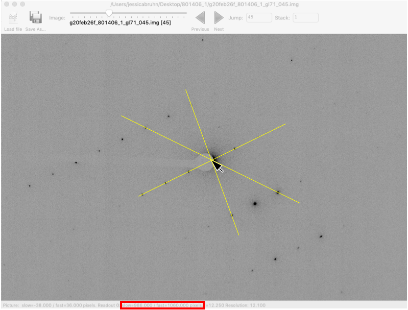
The first panel shows a low magnification image of the crystal target with the diffraction beam footprint indicated by the yellow circle. The second panel is a picture of the crystal as it would appear during the diffraction experiment with the stage tilt angle noted in yellow (note that some images are missing). The third panel shows the diffraction patterns generated during tilting. From these movies, we can see that crystal 801574_1 was poorly centered and moved out of the diffraction beam during collection.
Note about pedestal and offset
Data collected with the CETA/CETA-D cameras includes some pixels for which the recorded intensity value is negative. Many of these pixels likely still contain valuable information and therefore should not be entirely excluded from the data.
SMV format, a common format for X-ray crystallography diffraction images, does not allow for signed data (i.e. negative values). Because of this, Leginon adds an offset value to all pixels when converting to SMV format to make all values positive. Leginon also excludes negative values beyond a reasonable threshold.
Some data processing programs, such as DIALS, allow for signed data. Therefore, it can be beneficial to subtract a reasonable pedestal value, essentially resetting the zero point.
For data collected with Leginon, both the offset value applied (LEGINON_OFFSET), and a suggested pedestal value (IMAGE_PEDESTAL) are listed in the image metadata.
Import images
Correct interpretation of these images requires a special format class, installed as a plug-in for the dxtbx library. Installation only has to be done once, using this command:
dxtbx.install_format -u https://raw.githubusercontent.com/dials/dxtbx_ED_formats/master/FormatSMVCetaD_TUI.py
With that in place, you can start data processing, beginning with dataset 801406_1.
cd 801406_1
mkdir DIALS
cd DIALS
dials.import ../*.img panel.pedestal=980
Note
The suggested pedestal can be found by opening one of the images
with a text editor and finding the suggested pedestal value. This
value is provided by Leginon: 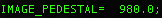 .
.
Find the beam centre
dials.image_viewer imported.expt
Opens the imported experiment in the image viewer
Turn off
 (note that the beam center from the image header
is not accurate)
(note that the beam center from the image header
is not accurate)It can be helpful to find the beam center using an image with good diffraction spots. Try moving the slider at the top of the window to image 45
Change Zoom to 50%. For weaker data you can also increase the brightness value
Move the mouse to the center of the direct beam, not the center of the beamstop. It can be helpful to find Friedel pairs and draw lines between them. The beam center should be in the center of Friedel pairs.
Make a note of the slow and fast beam center values at the bottom of the window (red box).
Close the viewer
Re-import with the correct beam center
dials.import ../*.img fast_slow_beam_centre=1059,988 panel.pedestal=980
Generate a mask for the beam center (optional)
dials.generate_mask imported.expt untrusted.circle=1059,988,100
The first two numbers are the beam center and the second is the diameter of the mask.
Find spots
dials.find_spots imported.expt gain=0.1 d_min=1.2 mask=pixels.mask\
  min_spot_size=2 max_separation=15 max_spot=5000
This step can be very time consuming when working with a new detector/data collection parameters. You want to make sure you are detecting enough spots corresponding to the lattice of interest to index your data and should adjust parameters until this is the case.
Here I have set the gain to 0.1, which is not the true gain for this detector. Modifying the gain here allows for the detection of more spots, but this will not impact integration step, which will use the correct gain (>26).
Note that I have adjusted the min and max spot sizes, as well as their separation.
I have also set the d_min to 1.2 Å to reduce the impact from high resolution spots not related to the lattice of interest (“zingers”).
In the log file (dials.find_spots.log), note the number of spots
found on each image. In this case, there are very few spots found in
the first 9 images:
Found 28 strong pixels on image 1
Found 8 strong pixels on image 2
Found 27 strong pixels on image 3
Found 1 strong pixels on image 4
Found 8 strong pixels on image 5
Found 160 strong pixels on image 6
Found 55 strong pixels on image 7
Found 67 strong pixels on image 8
Found 50 strong pixels on image 9
Found 276 strong pixels on image 10
Found 347 strong pixels on image 11
Found 598 strong pixels on image 12
Found 584 strong pixels on image 13
Found 483 strong pixels on image 14
Found 506 strong pixels on image 15
Found 327 strong pixels on image 16
Found 422 strong pixels on image 17
Found 286 strong pixels on image 18
Found 413 strong pixels on image 19
Found 483 strong pixels on image 20
Found 328 strong pixels on image 21
Found 142 strong pixels on image 22
Found 189 strong pixels on image 23
Found 140 strong pixels on image 24
Found 424 strong pixels on image 25
Found 1031 strong pixels on image 26
Found 735 strong pixels on image 27
Found 419 strong pixels on image 28
Found 374 strong pixels on image 29
Found 500 strong pixels on image 30
Found 670 strong pixels on image 31
Found 718 strong pixels on image 32
This is evident when opening the images with the image viewer:
dials.image_viewer imported.expt strong.refl
For now, just make a mental note that there are very few spots on images 1-9.
Indexing
dials.index imported.expt strong.refl detector.fix=distance
Fixing the detector distance is essential for electron diffraction data, as this generally cannot be refined at the same time as the unit cell.
Make sure that the camera length (distance) is carefully calibrated for your microscope as this value will not be refined by DIALS.
In the log file (dials.index.log), note the final RMSD_X and
RMSD_Y. The smaller the value the better. Generally, values lower than
3 are acceptable for electron diffraction data.
RMSDs by experiment:
+-------+--------+----------+----------+------------+
|   Exp |   Nref |   RMSD_X |   RMSD_Y |     RMSD_Z |
|    id |        |     (px) |     (px) |   (images) |
|-------+--------+----------+----------+------------|
|     0 |    988 |    1.205 |   1.8365 |    0.34229 |
+-------+--------+----------+----------+------------+
Also note the % of spots indexed. 79% is quite good for electron diffraction, but lower values (~30%) are still okay.
+------------+-------------+---------------+-------------+
|   Imageset |   # indexed |   # unindexed | % indexed   |
|------------+-------------+---------------+-------------|
|          0 |        1101 |           299 | 78.6%       |
+------------+-------------+---------------+-------------+
Find the Bravais lattice (optional)
dials.refine_bravais_settings indexed.refl indexed.expt detector.fix=distance
Potential lattices are listed.
Note the
Metric fitandrmsdvalues, as well as the recommended solutions:Chiral space groups corresponding to each Bravais lattice: aP: P1 mP: P2 P21 oP: P222 P2221 P21212 P212121 +------------+--------------+--------+--------------+----------+-----------+------------------------------------------+----------+----------+ | Solution | Metric fit | rmsd | min/max cc | #spots | lattice | unit_cell | volume | cb_op | |------------+--------------+--------+--------------+----------+-----------+------------------------------------------+----------+----------| | * 5 | 0.4889 | 0.08 | 0.763/0.873 | 990 | oP | 5.16 10.37 20.80 90.00 90.00 90.00 | 1112 | a,b,c | | * 4 | 0.4856 | 0.079 | 0.798/0.798 | 979 | mP | 5.17 10.36 20.81 90.00 90.26 90.00 | 1114 | a,b,c | | * 3 | 0.4889 | 0.074 | 0.763/0.763 | 996 | mP | 5.17 20.80 10.37 90.00 90.38 90.00 | 1115 | -a,-c,-b | | * 2 | 0.4718 | 0.068 | 0.873/0.873 | 1009 | mP | 10.37 5.17 20.80 90.00 90.41 90.00 | 1115 | -b,-a,-c | | * 1 | 0 | 0.062 | -/- | 989 | aP | 5.20 10.36 20.82 90.35 90.33 90.33 | 1121 | a,b,c | +------------+--------------+--------+--------------+----------+-----------+------------------------------------------+----------+----------+ * = recommended solution
Lattice choice is generally less straightforward for electron diffraction compared to X-ray data
When in doubt, process the data in P1 and determine the true symmetry after processing many datasets or after phasing the data (
ADDSYMin Platon is great for doing this)In this case, we know that the biotin crystal should be P212121, Solution #5 (primitive orthorhombic), but let’s just process in P1 to start with
Refine the geometry
dials.refine indexed.refl indexed.expt scan_varying=False detector.fix=distance
We start with a round of scan-static refinement. Although refinement is done during indexing, it is good practice to run a separate round to optimise the outlier rejection.
After that, we follow with scan-varying refinement
dials.refine refined.refl refined.expt scan_varying=True\
  detector.fix=all parameterisation.block_width=0.25\
  beam.fix="all in_spindle_plane out_spindle_plane *wavelength"\
  beam.force_static=False beam.smoother.absolute_num_intervals=1
We fix the detector position and orientation with
detector.fix=all, but now we are allowing the crystal unit cell, crystal orientation, and beam direction parameters to vary on a frame-by-frame basis withscan_varying=True.
Now RMSD_X and RMSD_Y have decreased significantly:
RMSDs by experiment:
+-------+--------+----------+----------+------------+
|   Exp |   Nref |   RMSD_X |   RMSD_Y |     RMSD_Z |
|    id |        |     (px) |     (px) |   (images) |
|-------+--------+----------+----------+------------|
|     0 |    890 |  0.79025 |   1.1428 |    0.24032 |
+-------+--------+----------+----------+------------+
This looks like a good model for the experiment, so we will continue on to integration.
Integration
dials.integrate refined.expt refined.refl d_min=0.8
We have set the high-resolution limit (
d_min) to 0.8 Å. Applying a resolution cutoff at integration speeds up later steps, especially scaling multiple datasets together. You want to set this to a smaller d-spacing limit than you expect for your dataset.
Scaling
dials.scale integrated.expt integrated.refl d_min=0.8
Though we will not directly use the output from scaling individual datasets, performing this step at this stage is helpful to assess the quality of the individual dataset.
Find the file dials.scale.html and open it in a web browser.
Note the useful statistics by resolution shells.
Keep in mind that merging statistics from incomplete and low multiplicity data are less reliable. It is generally best to wait to assess the final resolution cutoff until data from multiple crystals have been combined.
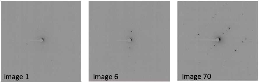
Scroll down the page a little and click
 . This brings up two
graphs. Let’s focus on the “Scale and Rmerge vs batch” plot:
. This brings up two
graphs. Let’s focus on the “Scale and Rmerge vs batch” plot:

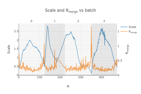
This plots the scale factor and Rmerge on a per frame (N) basis. Let’s focus on the orange Rmerge line (right axis).
Note that there is an uptick in Rmerge at the beginning and the end of the dataset. The higher Rmerge values at the start are likely due to the low number of spots that were found on those images, due to suboptimal centering. The uptick at the end is more likely to be due to radiation damage.
We will remove these high Rmerge frames after combining data from all four crystals.
Other datasets
Repeat this process for the other three datasets.
Hint, here are the import commands I used for each dataset:
- 801406_1
dials.import ../*.img fast_slow_beam_centre=1059,988 panel.pedestal=980- 801574_1
dials.import ../*.img fast_slow_beam_centre=1022,992 panel.pedestal=831- 802003_1
dials.import ../*.img fast_slow_beam_centre=1026,986 panel.pedestal=791- 810542_1
dials.import ../*.img fast_slow_beam_centre=1024,998 panel.pedestal=1619
Multi-dataset symmetry determination
We will run dials.cosym in a new directory alongside the dataset
directories
mkdir cosym
cd cosym
dials.cosym ../801406_1/DIALS/integrated.{expt,refl}\
  ../801574_1/DIALS/integrated.{expt,refl}\
  ../802003_1/DIALS/integrated.{expt,refl}\
  ../810542_1/DIALS/integrated.{expt,refl}
Towards the end of the log we see:
Scoring all possible sub-groups
+-------------------+----+--------------+----------+--------+--------+---------+--------------------+
| Patterson group   |    |   Likelihood |   NetZcc |   Zcc+ |   Zcc- |   delta | Reindex operator   |
|-------------------+----+--------------+----------+--------+--------+---------+--------------------|
| P 1 2/m 1         | ** |        0.715 |     3.19 |   9.43 |   6.24 |     0.3 | -a,-c,-b           |
| P m m m           |    |        0.149 |     7.46 |   7.46 |   0    |     0.3 | -a,-b,c            |
| P -1              |    |        0.071 |    -7.46 |   0    |   7.46 |     0   | -a,-b,c            |
| P 1 2/m 1         |    |        0.033 |    -1.75 |   6.25 |   7.99 |     0.3 | -b,-a,-c           |
| P 1 2/m 1         |    |        0.032 |    -1.77 |   6.23 |   8    |     0.2 | -a,-b,c            |
+-------------------+----+--------------+----------+--------+--------+---------+--------------------+
Best solution: P 1 2/m 1
Unit cell: (5.19032, 20.8498, 10.2916, 90, 90.2178, 90)
Reindex operator: -a,-c,-b
Laue group probability: 0.715
Laue group confidence: 0.636
Reindexing operators:
x,y,z: [0, 1, 2, 3]
Note that the suggested Patterson group is
P 1 2/m 1, notP m m mas we expect for biotin.This is likely due to the data being fed into dials.cosym being a little suboptimal.
We could force
dials.cosymto choose P212121 by addingspace_group=P212121to the above command and move on if we wanted, or we could improve the input files.
Excluding bad frames
Let’s improve the input files by going back and reprocess all datasets to exclude bad frames.
Remember the higher Rmerge we saw for certain frames in
dials.scale.htmlfor the first dataset? Let’s re-process each dataset and remove these “bad” frames.Start at the import step and exclude some of the bad frames:
- 801406_1
dials.import ../*.img fast_slow_beam_centre=1059,988 panel.pedestal=980 image_range=6,129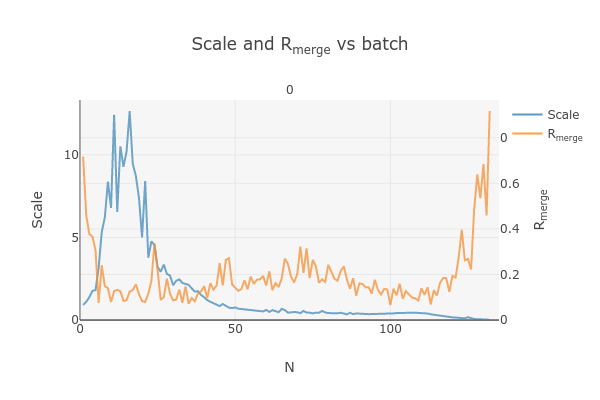
- 801574_1
dials.import ../*.img fast_slow_beam_centre=1022,992 panel.pedestal=831 image_range=1,101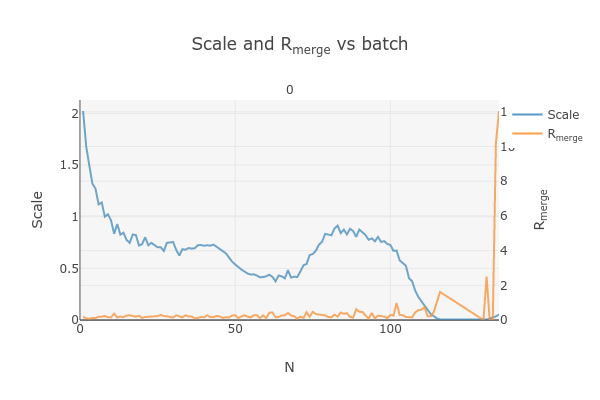
- 802003_1
dials.import ../*.img fast_slow_beam_centre=1026,986 panel.pedestal=791 image_range=1,126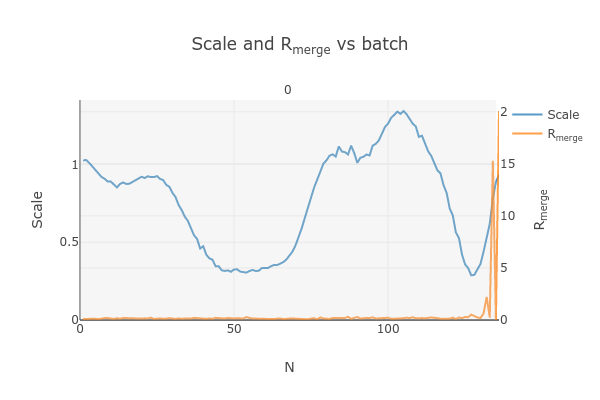
- 810542_1
dials.import ../*.img fast_slow_beam_centre=1024,998 panel.pedestal=1619 image_range=3,128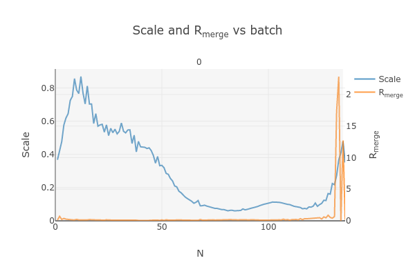
Process as before and re-run dials.cosym with the trimmed data:
+-------------------+-----+--------------+----------+--------+--------+---------+--------------------+
| Patterson group   |     |   Likelihood |   NetZcc |   Zcc+ |   Zcc- |   delta | Reindex operator   |
|-------------------+-----+--------------+----------+--------+--------+---------+--------------------|
| P m m m           | *** |        0.975 |     9.51 |   9.51 |   0    |     0.5 | a,b,c              |
| P 1 2/m 1         |     |        0.011 |     0.36 |   9.75 |   9.39 |     0.5 | -a,-c,-b           |
| P 1 2/m 1         |     |        0.007 |    -0.17 |   9.4  |   9.56 |     0.3 | -b,-a,-c           |
| P 1 2/m 1         |     |        0.007 |    -0.19 |   9.38 |   9.57 |     0.5 | a,b,c              |
| P -1              |     |        0.001 |    -9.51 |   0    |   9.51 |     0   | a,b,c              |
+-------------------+-----+--------------+----------+--------+--------+---------+--------------------+
Best solution: P m m m
Unit cell: (5.19159, 10.2937, 20.8531, 90, 90, 90)
Now the P m m m Patterson group is the most likely, as expected.
Scale the data together
Starting from the output of dials.cosym:
dials.scale symmetrized.expt symmetrized.refl nproc=8 d_min=0.8
The
d_min=0.8is not actually necessary because we only integrated to 0.8 Å.Open
dials.scale.html
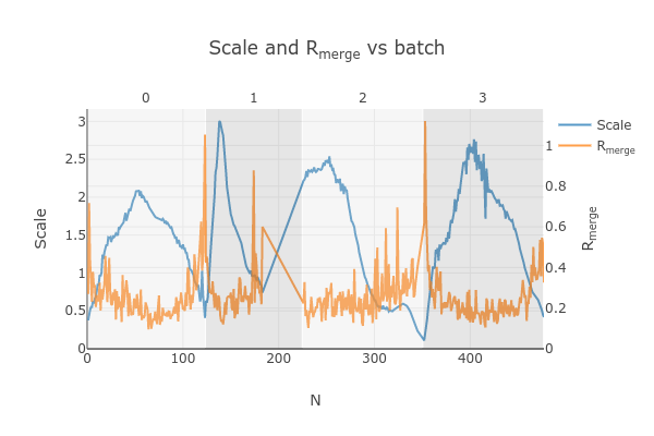
Note the increase in Rmerge part way through collection of dataset #1 (801574_1).
Let’s remove some of those images and see how that changes things:
dials.scale symmetrized.expt symmetrized.refl nproc=8 d_min=0.8 exclude_images="1:49:101"Here we have removed images 49-101 from dataset #1 as these had a fairly high Rmerge
            ----------Merging statistics by resolution bin----------

 d_max  d_min   #obs  #uniq   mult.  %comp       <I>  <I/sI>    r_mrg   r_meas    r_pim   r_anom   cc1/2   cc_ano
 20.86   2.17    941     92   10.23  97.87      19.6    29.0    0.104    0.109    0.032    0.085   0.994*   0.001
  2.17   1.72    943     69   13.67  98.57       8.8    22.8    0.158    0.164    0.044    0.074   0.989*  -0.263
  1.72   1.51    935     79   11.84 100.00       8.3    17.9    0.161    0.169    0.046    0.114   0.983*  -0.011
  1.51   1.37   1013     71   14.27 100.00       4.2    11.7    0.256    0.265    0.067    0.160   0.966*  -0.523
  1.37   1.27    865     63   13.73  96.92       3.5     9.4    0.277    0.288    0.076    0.225   0.942*   0.051
  1.27   1.20    970     76   12.76 100.00       3.2     8.3    0.307    0.322    0.091    0.213   0.816*  -0.612
  1.20   1.14    917     65   14.11 100.00       2.9     7.7    0.310    0.323    0.085    0.259   0.881*   0.306
  1.14   1.09    993     68   14.60 100.00       2.0     5.6    0.393    0.408    0.104    0.272   0.965*   0.167
  1.09   1.04    920     58   15.86 100.00       2.0     5.7    0.428    0.442    0.110    0.276   0.915*  -0.078
  1.04   1.01   1036     77   13.45  96.25       1.3     3.3    0.584    0.607    0.155    0.374   0.842*  -0.259
  1.01   0.98    856     61   14.03 100.00       1.1     2.4    0.622    0.647    0.166    0.520   0.735*   0.219
  0.98   0.95    931     69   13.49 100.00       0.6     1.5    0.873    0.910    0.246    0.628   0.495*  -0.306
  0.95   0.92    876     70   12.51 100.00       0.5     1.2    0.964    1.004    0.268    0.696   0.333*  -0.261
  0.92   0.90    751     62   12.11 100.00       0.3     0.9    1.146    1.194    0.326    0.805   0.491*  -0.324
  0.90   0.88    631     60   10.52 100.00       0.3     0.5    1.556    1.648    0.505    1.224   0.554*   0.219
  0.88   0.86    572     58    9.86  96.67       0.2     0.4    1.422    1.503    0.459    1.251   0.260  -0.050
  0.86   0.84    513     76    6.75 100.00       0.2     0.3    1.791    1.939    0.673    1.371   0.322*   0.051
  0.84   0.83    427     65    6.57  98.48       0.2     0.3    1.808    1.947    0.666    1.225   0.389*  -0.109
  0.83   0.81    423     62    6.82  95.38       0.2     0.2    2.817    3.054    1.078    1.996   0.099   0.173
  0.81   0.80    285     60    4.75  88.24       0.1     0.2    2.769    3.123    1.312    1.477  -0.003  -0.432
 20.85   0.80  15798   1361   11.61  98.27       3.4     7.1    0.246    0.257    0.071    0.205   0.988*  -0.111


Resolution limit suggested from CC½ fit (limit CC½=0.3): 0.83
Note that the completeness in the lower resolution shells have decreased a small amount. Let’s try adding back in some frames to boost the completeness back to 100% in the low-resolution shells:
dials.scale symmetrized.expt symmetrized.refl nproc=8 d_min=0.8 exclude_images="1:60:101"----------Merging statistics by resolution bin---------- d_max d_min #obs #uniq mult. %comp <I> <I/sI> r_mrg r_meas r_pim r_anom cc1/2 cc_ano 20.86 2.17 968 94 10.30 100.00 20.3 27.6 0.110 0.116 0.034 0.079 0.995* -0.080 2.17 1.72 961 71 13.54 100.00 9.1 13.3 0.164 0.170 0.045 0.075 0.989* -0.492 1.72 1.51 966 79 12.23 100.00 8.5 9.7 0.178 0.185 0.051 0.126 0.968* 0.074 1.51 1.37 1034 71 14.56 100.00 4.1 5.2 0.282 0.292 0.074 0.178 0.960* -0.365 1.37 1.27 891 65 13.71 100.00 3.1 3.6 0.332 0.345 0.090 0.288 0.906* -0.148 1.27 1.20 1003 76 13.20 100.00 2.8 3.0 0.364 0.379 0.103 0.267 0.708* -0.277 1.20 1.14 932 65 14.34 100.00 2.3 2.5 0.361 0.374 0.096 0.296 0.905* 0.020 1.14 1.09 1013 68 14.90 100.00 1.6 1.8 0.439 0.455 0.116 0.302 0.947* 0.242 1.09 1.04 937 58 16.16 100.00 1.5 1.7 0.477 0.493 0.121 0.361 0.812* -0.213 1.04 1.01 1081 80 13.51 100.00 0.9 1.0 0.672 0.699 0.180 0.393 0.739* 0.044 1.01 0.98 879 61 14.41 100.00 0.8 0.7 0.710 0.736 0.184 0.554 0.523* -0.264 0.98 0.95 951 69 13.78 100.00 0.5 0.4 0.917 0.953 0.249 0.481 0.571* -0.105 0.95 0.92 897 70 12.81 100.00 0.4 0.4 1.082 1.124 0.294 0.796 0.386* -0.125 0.92 0.90 760 62 12.26 100.00 0.2 0.2 1.439 1.500 0.409 0.920 0.346* -0.262 0.90 0.88 642 60 10.70 100.00 0.2 0.2 1.777 1.866 0.544 1.208 0.514* 0.190 0.88 0.86 593 61 9.72 100.00 0.2 0.1 1.706 1.827 0.605 1.294 -0.290 -0.089 0.86 0.84 538 76 7.08 100.00 0.1 0.1 2.044 2.195 0.744 1.534 0.289* -0.067 0.84 0.83 436 65 6.71 98.48 0.1 0.1 2.146 2.314 0.799 1.353 0.363* 0.005 0.83 0.81 432 62 6.97 95.38 0.2 0.1 3.472 3.752 1.306 1.794 0.137 0.052 0.81 0.80 291 60 4.85 88.24 0.1 0.1 4.041 4.519 1.851 1.350 0.128 -0.490 20.85 0.80 16205 1373 11.80 99.13 3.3 4.2 0.255 0.266 0.072 0.201 0.988* -0.127 Resolution limit suggested from CC½ fit (limit CC½=0.3): 0.85
This looks a lot better in terms of completeness.
Looking at
dials.scale.htmlwe can probably improve this a little by removing some images from the end of dataset #2
So, we run
dials.scale symmetrized.expt symmetrized.refl nproc=8 d_min=0.8 exclude_images="1:60:101" exclude_images="2:121:126"----------Merging statistics by resolution bin---------- d_max d_min #obs #uniq mult. %comp <I> <I/sI> r_mrg r_meas r_pim r_anom cc1/2 cc_ano 20.86 2.17 954 94 10.15 100.00 20.4 27.4 0.105 0.110 0.033 0.077 0.993* -0.028 2.17 1.72 943 71 13.28 100.00 9.1 13.5 0.161 0.168 0.044 0.075 0.991* -0.079 1.72 1.51 957 79 12.11 100.00 8.4 9.9 0.178 0.186 0.051 0.126 0.971* 0.053 1.51 1.37 1017 71 14.32 100.00 4.1 5.3 0.272 0.282 0.073 0.177 0.956* -0.203 1.37 1.27 885 65 13.62 100.00 3.1 3.7 0.334 0.347 0.090 0.288 0.908* -0.017 1.27 1.20 988 76 13.00 100.00 2.7 3.1 0.359 0.375 0.102 0.265 0.722* -0.331 1.20 1.14 914 65 14.06 100.00 2.3 2.6 0.352 0.366 0.096 0.295 0.900* 0.192 1.14 1.09 994 68 14.62 100.00 1.6 1.8 0.436 0.452 0.116 0.304 0.870* 0.185 1.09 1.04 920 58 15.86 100.00 1.4 1.8 0.475 0.490 0.122 0.364 0.761* -0.397 1.04 1.01 1072 80 13.40 100.00 0.9 1.0 0.637 0.663 0.173 0.394 0.775* -0.137 1.01 0.98 869 61 14.25 100.00 0.8 0.8 0.714 0.741 0.186 0.560 0.608* -0.175 0.98 0.95 942 69 13.65 100.00 0.4 0.5 0.921 0.957 0.253 0.486 0.755* -0.151 0.95 0.92 888 70 12.69 100.00 0.4 0.4 1.059 1.101 0.290 0.798 0.289* -0.155 0.92 0.90 746 62 12.03 100.00 0.2 0.2 1.471 1.534 0.421 0.911 0.101 -0.218 0.90 0.88 629 60 10.48 100.00 0.2 0.2 1.635 1.719 0.507 1.189 0.550* 0.023 0.88 0.86 584 61 9.57 100.00 0.2 0.1 1.679 1.800 0.602 1.315 -0.212 -0.147 0.86 0.84 529 76 6.96 100.00 0.1 0.1 2.107 2.272 0.790 1.577 0.223 -0.078 0.84 0.83 429 65 6.60 98.48 0.1 0.1 2.101 2.274 0.802 1.318 0.569* -0.058 0.83 0.81 426 62 6.87 95.38 0.2 0.1 2.047 2.232 0.808 1.842 0.220 0.046 0.81 0.80 287 60 4.78 88.24 0.1 0.1 4.537 5.104 2.145 1.340 0.100 -0.650 20.85 0.80 15973 1373 11.63 99.13 3.3 4.2 0.248 0.259 0.071 0.199 0.991* -0.148
This looks reasonably good
Export the data
We export the scaled, unmerged dataset to MTZ format:
dials.export scaled.refl scaled.expt mtz.hklout=biotin_P222.mtz
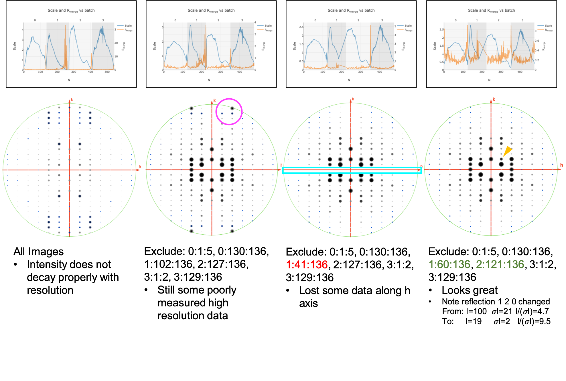
It can be helpful to open the
biotin_P222.mtzfile in CCP4’s ViewHKL programYou want to see a nice decay of intensities, with more intense spots in the middle and lower intensity spots towards the edges. You also want to make sure that you see some variation in your reflection intensities. They should not all be the same value as can happen when scaling goes poorly.
Now we want to convert to SHELX format for structure solution
xia2.to_shelx biotin_P222.mtz biotin_P222 CHNOS
Solve the structure
Prepare an .ins file for SHELXT or SHELXD by either running XPREP or
manually editing the .ins file as shown below:
TITL biotin_P212121 in P2(1)2(1)2(1)
CELL 0.02501   5.19177  10.29400  20.84910  90.0000  90.0000  90.0000
ZERR    4.00   0.00104   0.00206   0.00417   0.0000   0.0000   0.0000
LATT -1
SYMM 0.5-X, -Y, 0.5+Z
SYMM -X, 0.5+Y, 0.5-Z
SYMM 0.5+X, 0.5-Y, -Z
SFAC C H N O S
UNIT 40 64 8 12 4
FIND    10
PLOP    14    17    19
MIND 1.0 -0.1
NTRY 1000
HKLF 4
END
Now phase the data:
shelxt biotin_P212121
If you are processing a more challenging organic small molecule dataset you could try this:
shelxt biotin_P212121 -y -m1000
If this fails (it should not fail for biotin as this is really high-quality data), you could try SHELXD, which has been more successful in phasing challenging datasets here at NIS:
shelxd biotin_P212121
Note that you have to have the space group correct for SHELXD to work.
When you are having difficulties, try solving this in P1 and figuring out the proper space group once you have a solution with
ADDSYMin PLATON.It can help to increase the
NTRY. Try 50000 for challenging cases.
If SHELXD fails, I usually go back and remove more datasets/bad images and try again.
If that fails, you can try molecular replacement with PHASER.
Note that you will need merged data and an R-free set. I recommend using
dials.mergeand thenfreerflagin CCP4.The model used needs to be very accurate in terms of RMSD with the final structure.
When defining the contents of the ASU, try setting this to 2% solvent content.
If you are still struggling, I recommend going back and collecting more data or growing better crystals. Sometimes one crystal will diffract to much higher resolution than the others. For challenging cases, we have collected data from ~200 crystals just to find ~5 good ones to combine.
Good luck!