
Multi-crystal analysis with DIALS and xia2.multiplex
Introduction
The actual processing of multi-crystal data is essentially no different to processing regular rotation data in the first instance - though there are some potential differences in how you handle the data, by and large the process for an individual sweep is straightforward. The work comes in identifying which subsets of data (e.g. which crystals, or subsets of data from crystals) to merge into the final data set. This tutorial covers the basics of how to use DIALS tools to make these choices.
One particular issue with multi-crystal data processing is the “bookkeeping” i.e. keeping track of individual data sets, which can become cumbersome when the numbers are large. This tutorial is aimed at helping you to use the tools at your disposal to process such data with the minimum of 🤯.
The aim of the tutorial is to introduce you to tools for symmetry determination, incremental scaling and data elimination such that you could use them during experimental beam time.
Data
For this tutorial the data kindly provided from a CCP4 School at SPring
8 will be used - in particular
the 31 data sets included in bl32xu_group2_data.tar.xz. These are
recorded using the zoo system with an Eiger 9M detector, and appear
in the data files as 3,100 images which we have to interpret as 31 x
100 image @ 0.1° / frame data sets. The data are from small samples of
tetragonal lysozyme (unit cell ~ 78, 78, 38, 90, 90, 90, space group
P43212), though we won’t use that information from the outset.
The mode of data collection makes these data a little “special” so when
importing care must be taken to treat the 31 x 100 image data sets as
different data sets: in dials.import using image_range=1,100
etc. is necessary. The data were taken from a single loop, which was
raster scanned to identify the sample positions then collected using the
ZOO system:
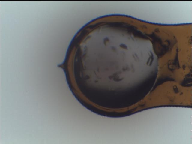
Loop image
Bookkeeping
This process will involve processing dozens of data sets, will create hundreds of files and will involve running similar looking scaling tasks on several occasions so care will need to be taken on how you organise yourself.
I’ve chosen to present the processing as directories sweep00 to
sweep30 (i.e. 31 directories, using computer counting) and then
combine0-9 for combining first 10, combine0-19 for first 20 etc.
Any other organisation will do, but these need to be consistent.
Process
The first step is to integrate the data we have - without making any assumptions. For this the following bash “spell” is appropriate:
for ((j=0;j<31;j++));
do
  mkdir sweep-$(printf %02d $j)
  cd sweep-$(printf %02d $j)
  dials.import ../../*master* image_range=$((100 * j + 1)),$((100 * j + 100))
  dials.find_spots imported.expt
  dials.index imported.expt strong.refl
  dials.refine indexed.expt indexed.refl
  dials.integrate refined.expt refined.refl
  cd -
done
This will import and process each 100 image block and really
demonstrates how shell scripting can be powerful. In “real” data
collection each data set would probably have a different filename, so
the only change would be altering the dials.import command.
This will generate 31 × {integrated.refl,integrated.expt} pairs that
are the real input to this process. For this tutorial we will work on
the first 10, then add the next ten etc. demonstrating the incremental
approach to combining the data.
Sets 0-9
First,
$ mkdir combine0-9
$ cd combine0-9
to give us somewhere to work for this - we will first use the
dials.cosym tool to bring all the data together, estimate the
symmetry and then prepare the data for scaling. This is run with:
combine0-9 $ dials.cosym ../sweep-0*/integrated.*
This takes the following files
combine0-9 $ ls ../sweep-0*/integrated.*
../sweep-00/integrated.expt ../sweep-05/integrated.expt
../sweep-00/integrated.refl ../sweep-05/integrated.refl
../sweep-01/integrated.expt ../sweep-06/integrated.expt
../sweep-01/integrated.refl ../sweep-06/integrated.refl
../sweep-02/integrated.expt ../sweep-07/integrated.expt
../sweep-02/integrated.refl ../sweep-07/integrated.refl
../sweep-03/integrated.expt ../sweep-08/integrated.expt
../sweep-03/integrated.refl ../sweep-08/integrated.refl
../sweep-04/integrated.expt ../sweep-09/integrated.expt
../sweep-04/integrated.refl ../sweep-09/integrated.refl
and:
Maps all crystals back to P1,
Checks them for consistency in unit cell,
Determines the maximum possible lattice symmetry and lists of possible operations,
Tests all operations against all pairs of data sets,
Decides those that apply which are space group operations - those which do not apply are “twinning operations” i.e. indexing ambiguity,
Resolves ambiguity and output data consistently indexed in the correct space group.
In this case the correct space group is the same as the lattice symmetry i.e. P4/mmm, so there is no residual ambiguity. The output gives an indication of this:
Best number of dimensions: 6
Using 6 dimensions for analysis
Principal component analysis:
Explained variance: 0.0015, 0.0013, 0.0012, 0.00078, 0.00062, 0.00047
Explained variance ratio: 0.25, 0.22, 0.2, 0.13, 0.11, 0.081
Scoring individual symmetry elements
+--------------+--------+------+-----+-----------------+
|   likelihood |   Z-CC |   CC |     | Operator        |
|--------------+--------+------+-----+-----------------|
|        0.947 |   9.95 | 0.99 | *** | 4 |(1, 0, 0)    |
|        0.947 |   9.95 | 0.99 | *** | 4^-1 |(1, 0, 0) |
|        0.947 |   9.94 | 0.99 | *** | 2 |(1, 0, 0)    |
|        0.947 |   9.94 | 0.99 | *** | 2 |(0, 1, 0)    |
|        0.946 |   9.92 | 0.99 | *** | 2 |(0, 0, 1)    |
|        0.947 |   9.93 | 0.99 | *** | 2 |(0, 1, 1)    |
|        0.947 |   9.94 | 0.99 | *** | 2 |(0, -1, 1)   |
+--------------+--------+------+-----+-----------------+
Scoring all possible sub-groups
+-------------------+-----+--------------+----------+--------+--------+---------+--------------------+
| Patterson group   |     |   Likelihood |   NetZcc |   Zcc+ |   Zcc- |   delta | Reindex operator   |
|-------------------+-----+--------------+----------+--------+--------+---------+--------------------|
| P 4/m m m         | *** |            1 |     9.94 |   9.94 |   0    |     0.1 | b,c,a              |
| P 4/m             |     |            0 |     0.01 |   9.94 |   9.93 |     0.1 | b,c,a              |
| C m m m           |     |            0 |     0    |   9.94 |   9.94 |     0.1 | b+c,-b+c,a         |
| P m m m           |     |            0 |    -0.01 |   9.93 |   9.94 |     0.1 | a,b,c              |
| C 1 2/m 1         |     |            0 |     0    |   9.94 |   9.94 |     0.1 | b+c,-b+c,a         |
| P 1 2/m 1         |     |            0 |     0    |   9.94 |   9.94 |     0.1 | -b,-a,-c           |
| P 1 2/m 1         |     |            0 |    -0    |   9.94 |   9.94 |     0.1 | a,b,c              |
| C 1 2/m 1         |     |            0 |    -0    |   9.93 |   9.94 |     0.1 | b-c,b+c,a          |
| P 1 2/m 1         |     |            0 |    -0.02 |   9.92 |   9.94 |     0.1 | -a,-c,-b           |
| P -1              |     |            0 |    -9.94 |   0    |   9.94 |     0   | a,b,c              |
+-------------------+-----+--------------+----------+--------+--------+---------+--------------------+
Best solution: P 4/m m m
Unit cell: (79.2189, 79.2189, 37.2723, 90, 90, 90)
Reindex operator: b,c,a
Laue group probability: 1.000
Laue group confidence: 1.000
Reindexing operators:
x,y,z: [0, 1, 2, 3, 4, 5, 6, 7, 8, 9]
and a dials.cosym.html is generated, which can be opened with a browser
(e.g. firefox dials.cosym.html) and graphically illustrates some of the
analysis. The data are now prepared for scaling, and we can scale them with a
standard command:
$ dials.scale symmetrized.*
It is critical to note here, that though we have combined the data from 10 sweeps into two files - the data retain their original identity. This means that in the files they are still 10 sweeps.
The first scaling output has:
Resolution limit suggested from CC½ fit (limit CC½=0.3): 1.42

            -------------Summary of merging statistics--------------

                                            Suggested   Low    High  Overall
High resolution limit                           1.42    3.87    1.42    1.09
Low resolution limit                           79.22   79.34    1.45   79.22
Completeness                                   98.8    98.9    98.7    85.1
Multiplicity                                    7.4     7.2     7.7     5.9
I/sigma                                         7.4    34.4     0.3     4.0
Rmerge(I)                                     0.124   0.072   2.275   0.156
Rmerge(I+/-)                                  0.113   0.063   2.201   0.141
Rmeas(I)                                      0.134   0.078   2.444   0.170
Rmeas(I+/-)                                   0.130   0.072   2.525   0.163
Rpim(I)                                       0.048   0.028   0.866   0.064
Rpim(I+/-)                                    0.061   0.033   1.200   0.080
CC half                                       0.994   0.993   0.263   0.994
Anomalous completeness                         95.4    93.6    96.3    70.9
Anomalous multiplicity                          4.0     4.4     4.1     3.4
Anomalous correlation                         0.165   0.278  -0.039   0.125
Anomalous slope                               0.275
dF/F                                          0.095
dI/s(dI)                                      0.421
Total observations                           167233    9155    8507  247651
Total unique                                  22555    1278    1104   42048
indicating that we have an almost complete data set already, though the
high resolution limit is a little enthusiastic. Setting it for this
analysis with e.g. d_min=1.45 will allow focus on the key point of
isomorphism etc. - to this limit we have:
                                             Overall    Low     High
High resolution limit                           1.45    3.94    1.45
Low resolution limit                           79.22   79.34    1.48
Completeness                                   98.8    98.9    98.7
Multiplicity                                    7.4     7.1     7.7
I/sigma                                         7.7    34.0     0.4
Rmerge(I)                                     0.122   0.072   1.676
Rmerge(I+/-)                                  0.111   0.063   1.588
Rmeas(I)                                      0.131   0.078   1.801
Rmeas(I+/-)                                   0.127   0.072   1.823
Rpim(I)                                       0.047   0.028   0.637
Rpim(I+/-)                                    0.060   0.033   0.864
CC half                                       0.995   0.992   0.370
Anomalous completeness                         95.4    93.6    96.0
Anomalous multiplicity                          4.0     4.4     4.1
Anomalous correlation                         0.145   0.258  -0.087
Anomalous slope                               0.292
dF/F                                          0.094
dI/s(dI)                                      0.439
Total observations                           158400    8650    8072
Total unique                                  21401    1212    1054
and it is well worth taking a look around dials.scale.html.
Sets 10-19
This time around we are going to take what we have already processed above and add 10 more data sets to it.
First,
combine0-9  $ mkdir ../combine0-19
combine0-19 $ cd ../combine0-19
Then:
combine0-19 $ dials.cosym ../combine0-9/scaled.* ../sweep-1*/integrated.*
Which is using these files:
combine0-19 $ ls ../combine0-9/scaled.* ../sweep-1*/integrated.*
../combine0-9/scaled.expt   ../sweep-14/integrated.refl
../combine0-9/scaled.refl   ../sweep-15/integrated.expt
../sweep-10/integrated.expt ../sweep-15/integrated.refl
../sweep-10/integrated.refl ../sweep-16/integrated.expt
../sweep-11/integrated.expt ../sweep-16/integrated.refl
../sweep-11/integrated.refl ../sweep-17/integrated.expt
../sweep-12/integrated.expt ../sweep-17/integrated.refl
../sweep-12/integrated.refl ../sweep-18/integrated.expt
../sweep-13/integrated.expt ../sweep-18/integrated.refl
../sweep-13/integrated.refl ../sweep-19/integrated.expt
../sweep-14/integrated.expt ../sweep-19/integrated.refl
This will take the scaled output from the previous step, and the next 10 processed sweeps, and combine them as before:
Best solution: P 4/m m m
Unit cell: (79.227, 79.227, 37.2723, 90, 90, 90)
Reindex operator: b,c,a
Laue group probability: 1.000
Laue group confidence: 1.000
Reindexing operators:
x,y,z: [0, 1, 2, 3, 4, 5, 6, 7, 8, 9, 10, 11, 12, 13, 14, 15, 16, 17, 18, 19]
Running through scaling as before, setting a 1.45 Å resolution limit, we see:
Resolution limit suggested from CC½ fit (limit CC½=0.3): 1.48

            -------------Summary of merging statistics--------------

                                            Suggested   Low    High  Overall
High resolution limit                           1.48    4.02    1.48    1.45
Low resolution limit                           79.22   79.33    1.51   79.22
Completeness                                  100.0    99.7    99.9   100.0
Multiplicity                                   14.8    14.5    15.2    14.9
I/sigma                                         9.3    38.0     0.7     8.8
Rmerge(I)                                     0.149   0.081   2.793   0.155
Rmerge(I+/-)                                  0.142   0.073   2.749   0.148
Rmeas(I)                                      0.154   0.084   2.892   0.161
Rmeas(I+/-)                                   0.151   0.078   2.942   0.158
Rpim(I)                                       0.039   0.021   0.728   0.041
Rpim(I+/-)                                    0.052   0.026   1.018   0.054
CC half                                       0.997   0.996   0.151   0.997
Anomalous completeness                         99.9    99.9    99.9    99.9
Anomalous multiplicity                          8.0     8.7     8.0     8.0
Anomalous correlation                         0.213   0.371   0.080   0.240
Anomalous slope                               0.338
dF/F                                          0.086
dI/s(dI)                                      0.549
Total observations                           301412   16640   15140  321968
Total unique                                  20324    1149     995   21649
i.e. somehow adding more data has reduced the overall resolution
limit. Looking at the plots in dials.scale.html we see that the
R-merge value is rather high for some of the sweeps indicating that they
do not agree well with the overall data. R-merge is however not a good
basis for exclusion of data - for that we have ΔCC½.
With:
combine0-19 $ dials.compute_delta_cchalf scaled.*
we may calculate the effect of adding individual data sets to the data as a whole - if this effect is negative then that data set should probably not be included. The tool outputs:
Dataset: 15, ΔCC½: -3.625
Dataset: 12, ΔCC½: -1.055
Dataset: 14, ΔCC½: -0.599
Dataset: 9, ΔCC½: -0.254
Dataset: 1, ΔCC½: 0.056
Dataset: 13, ΔCC½: 0.463
Dataset: 5, ΔCC½: 0.508
Dataset: 7, ΔCC½: 0.527
Dataset: 0, ΔCC½: 0.528
Dataset: 17, ΔCC½: 0.631
Dataset: 2, ΔCC½: 0.758
Dataset: 10, ΔCC½: 0.770
Dataset: 18, ΔCC½: 0.773
Dataset: 19, ΔCC½: 0.843
Dataset: 4, ΔCC½: 0.854
Dataset: 16, ΔCC½: 0.898
Dataset: 6, ΔCC½: 0.931
Dataset: 8, ΔCC½: 1.192
Dataset: 3, ΔCC½: 1.444
Dataset: 11, ΔCC½: 1.705

mean delta_cc_half 0.3674101744536096
stddev delta_cc_half 1.1112402970091422
cutoff value: -4.0775510135829585
Suggesting that dataset 15 looks to agree rather poorly. This may be
excluded from scaling with exclude_datasets=15 giving:
                                            Suggested   Low    High  Overall
High resolution limit                           1.46    3.95    1.46    1.45
Low resolution limit                           79.21   79.32    1.48   79.21
Completeness                                  100.0    99.8    99.9   100.0
Multiplicity                                   14.1    13.8    14.7    14.1
I/sigma                                         8.9    38.1     0.6     8.8
Rmerge(I)                                     0.139   0.079   2.238   0.140
Rmerge(I+/-)                                  0.131   0.071   2.185   0.132
Rmeas(I)                                      0.144   0.082   2.322   0.145
Rmeas(I+/-)                                   0.141   0.076   2.346   0.142
Rpim(I)                                       0.038   0.021   0.602   0.038
Rpim(I+/-)                                    0.050   0.026   0.831   0.050
CC half                                       0.996   0.996   0.482   0.997
Anomalous completeness                         99.9    99.9    99.8    99.9
Anomalous multiplicity                          7.6     8.3     7.7     7.6
Anomalous correlation                         0.196   0.153  -0.067   0.222
Anomalous slope                               0.316
dF/F                                          0.088
dI/s(dI)                                      0.522
Total observations                           300879   16563   15320  304888
Total unique                                  21363    1203    1040   21637
This gives a small overall improvement in \(R_\textrm{pim}\) - we may
exclude all negative contribution data sets with exclude_dataset=15,12,14,9
giving:
                                             Overall    Low     High
High resolution limit                           1.45    3.94    1.45
Low resolution limit                           79.18   79.29    1.48
Completeness                                   99.6    99.2    99.2
Multiplicity                                   11.9    11.6    12.4
I/sigma                                         8.7    36.9     0.6
Rmerge(I)                                     0.129   0.077   1.534
Rmerge(I+/-)                                  0.121   0.069   1.490
Rmeas(I)                                      0.135   0.081   1.602
Rmeas(I+/-)                                   0.132   0.075   1.622
Rpim(I)                                       0.038   0.023   0.448
Rpim(I+/-)                                    0.050   0.028   0.619
CC half                                       0.996   0.995   0.482
Anomalous completeness                         98.8    97.8    99.1
Anomalous multiplicity                          6.4     7.0     6.5
Anomalous correlation                         0.205   0.250   0.041
Anomalous slope                               0.315
dF/F                                          0.092
dI/s(dI)                                      0.519
Total observations                           255800   14071   13145
Total unique                                  21540    1212    1061
It is critical to note that once a data set has been excluded it stays
excluded if you work from the output of dials.scale. In the process
we are working through here, this is good, as you have a realistic idea of
how the data look, but once you’re done collecting data it may be worth
revisiting this.
Sets 20-29
Now we add the next batch of 10 data sets to the 16 we kept from the run before:
combine0-19 $ mkdir ../combine0-29
combine0-29 $ cd ../combine0-29

combine0-29 $ dials.cosym ../combine0-19/scaled.* ../sweep-2*/integrated.*
combine0-29 $ dials.scale symmetrized.* d_min=1.45
giving
                                             Overall    Low     High
High resolution limit                           1.45    3.94    1.45
Low resolution limit                           79.19   79.31    1.48
Completeness                                  100.0    99.8   100.0
Multiplicity                                   19.2    18.8    19.9
I/sigma                                         9.5    40.0     0.7
Rmerge(I)                                     0.193   0.088   5.094
Rmerge(I+/-)                                  0.186   0.081   5.054
Rmeas(I)                                      0.198   0.090   5.239
Rmeas(I+/-)                                   0.196   0.085   5.331
Rpim(I)                                       0.045   0.020   1.180
Rpim(I+/-)                                    0.060   0.025   1.639
CC half                                       0.996   0.996   0.231
Anomalous completeness                        100.0   100.0   100.0
Anomalous multiplicity                         10.3    11.3    10.5
Anomalous correlation                         0.145   0.389   0.046
Anomalous slope                               0.366
dF/F                                          0.089
dI/s(dI)                                      0.626
Total observations                           415898   22943   21222
Total unique                                  21636    1220    1065
Then
combine0-29 $ dials.compute_delta_cchalf scaled.*
giving:
Dataset: 18, ΔCC½: -10.148
Dataset: 19, ΔCC½: -0.252
Dataset: 23, ΔCC½: -0.128
Dataset: 22, ΔCC½: -0.023
Dataset: 21, ΔCC½: 0.054
Dataset: 5, ΔCC½: 0.153
Dataset: 25, ΔCC½: 0.153
Dataset: 16, ΔCC½: 0.240
Dataset: 7, ΔCC½: 0.246
Dataset: 14, ΔCC½: 0.272
Dataset: 9, ΔCC½: 0.300
Dataset: 2, ΔCC½: 0.319
Dataset: 1, ΔCC½: 0.335
Dataset: 0, ΔCC½: 0.399
Dataset: 11, ΔCC½: 0.400
Dataset: 4, ΔCC½: 0.461
Dataset: 12, ΔCC½: 0.666
Dataset: 13, ΔCC½: 0.674
Dataset: 6, ΔCC½: 0.724
Dataset: 15, ΔCC½: 0.749
Dataset: 24, ΔCC½: 0.824
Dataset: 8, ΔCC½: 1.097
Dataset: 17, ΔCC½: 1.187
Dataset: 3, ΔCC½: 1.225
Dataset: 20, ΔCC½: 1.321
Dataset: 10, ΔCC½: 1.422
This is probably a good indicator that set 18 is not good so let’s remove it:
combine0-29 $ dials.scale symmetrized.* d_min=1.45 exclude_dataset=18
Giving:
                                             Overall    Low     High
High resolution limit                           1.45    3.94    1.45
Low resolution limit                           79.21   79.33    1.48
Completeness                                  100.0    99.8   100.0
Multiplicity                                   18.5    18.1    19.2
I/sigma                                         9.5    40.2     0.7
Rmerge(I)                                     0.164   0.081   3.042
Rmerge(I+/-)                                  0.157   0.074   3.004
Rmeas(I)                                      0.169   0.083   3.127
Rmeas(I+/-)                                   0.165   0.077   3.169
Rpim(I)                                       0.038   0.019   0.699
Rpim(I+/-)                                    0.051   0.023   0.973
CC half                                       0.997   0.996   0.359
Anomalous completeness                        100.0   100.0   100.0
Anomalous multiplicity                          9.9    10.9    10.1
Anomalous correlation                         0.226   0.321   0.089
Anomalous slope                               0.365
dF/F                                          0.089
dI/s(dI)                                      0.616
Total observations                           400223   22084   20368
Total unique                                  21639    1221    1063
By this point there is a good chance you are becoming “snow blind” from all the numbers in the output and they cease to have meaning - and you could not be blamed for this. Once you have complete data which appears to be internally isomorphous, actually attempting structure solution on the processed data will be key, e.g. trying to find the heavy atom substructure or similar, as a more robust measure.
Explorations of Reciprocal Space
So far the process has been very focussed on getting the processing done
with minimal exploration. There is however something to explore here -
loading the data we have processed in
dials.reciprocal_lattice_viewer will give a real insight into what
the data sets are adding:
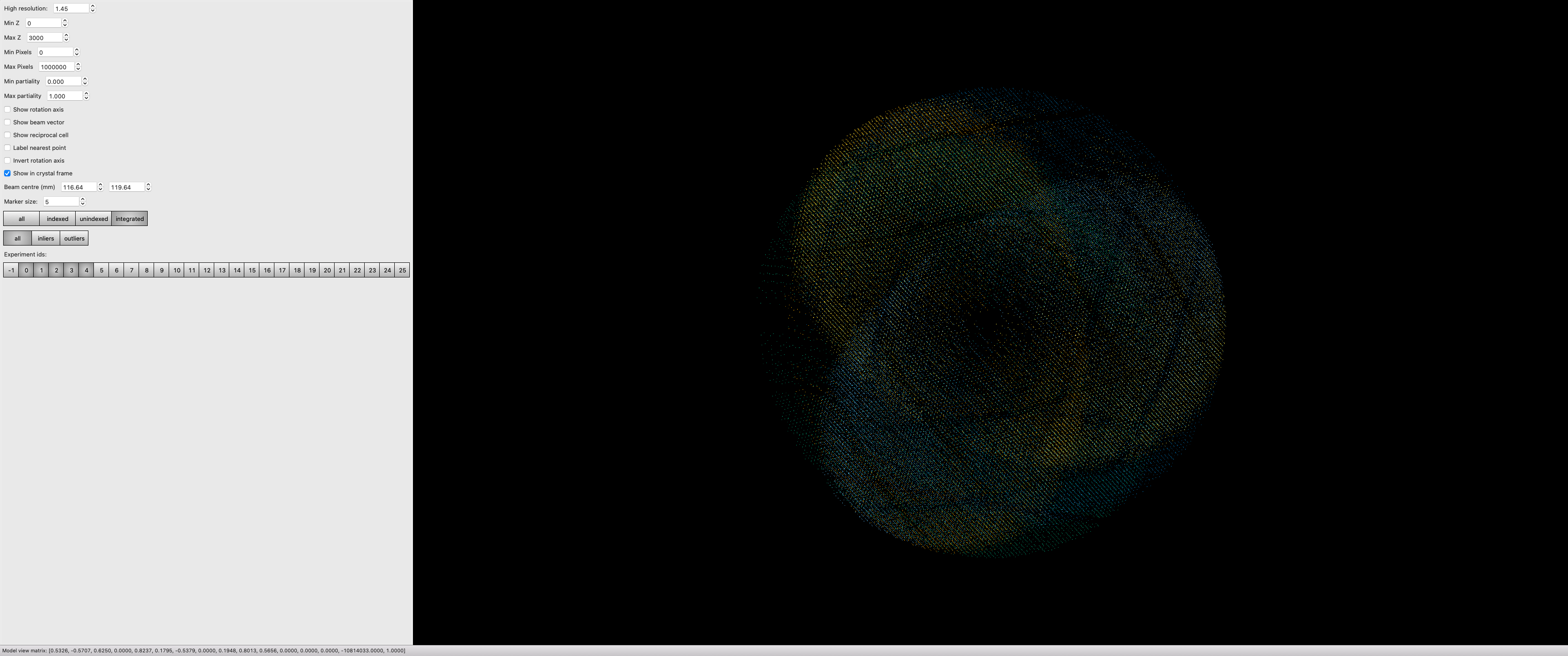
combine0-29 $ dials.reciprocal_lattice_viewer scaled.*
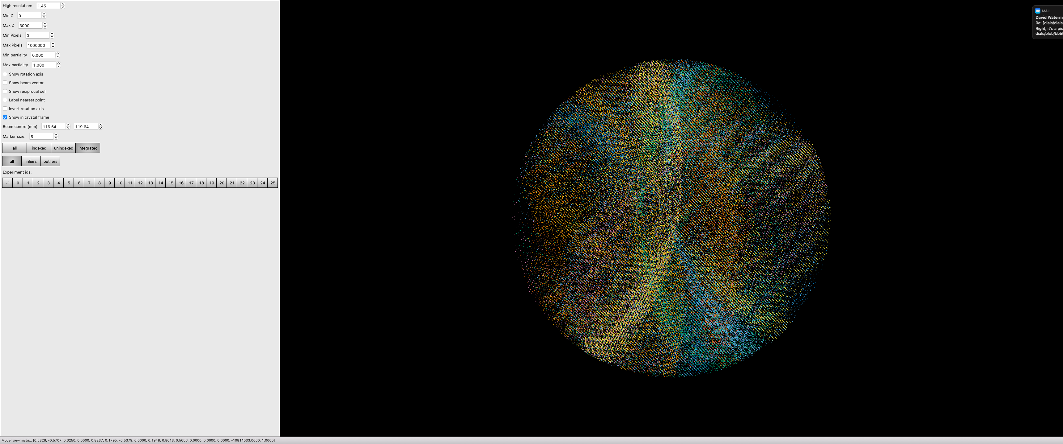
Note here we are looking in the crystal frame (see toggle in the tool panel), a sensible resolution limit has been set, and the integrated data are being projected. You can also “switch on” individual data sets to really see what bits of reciprocal space we are adding.
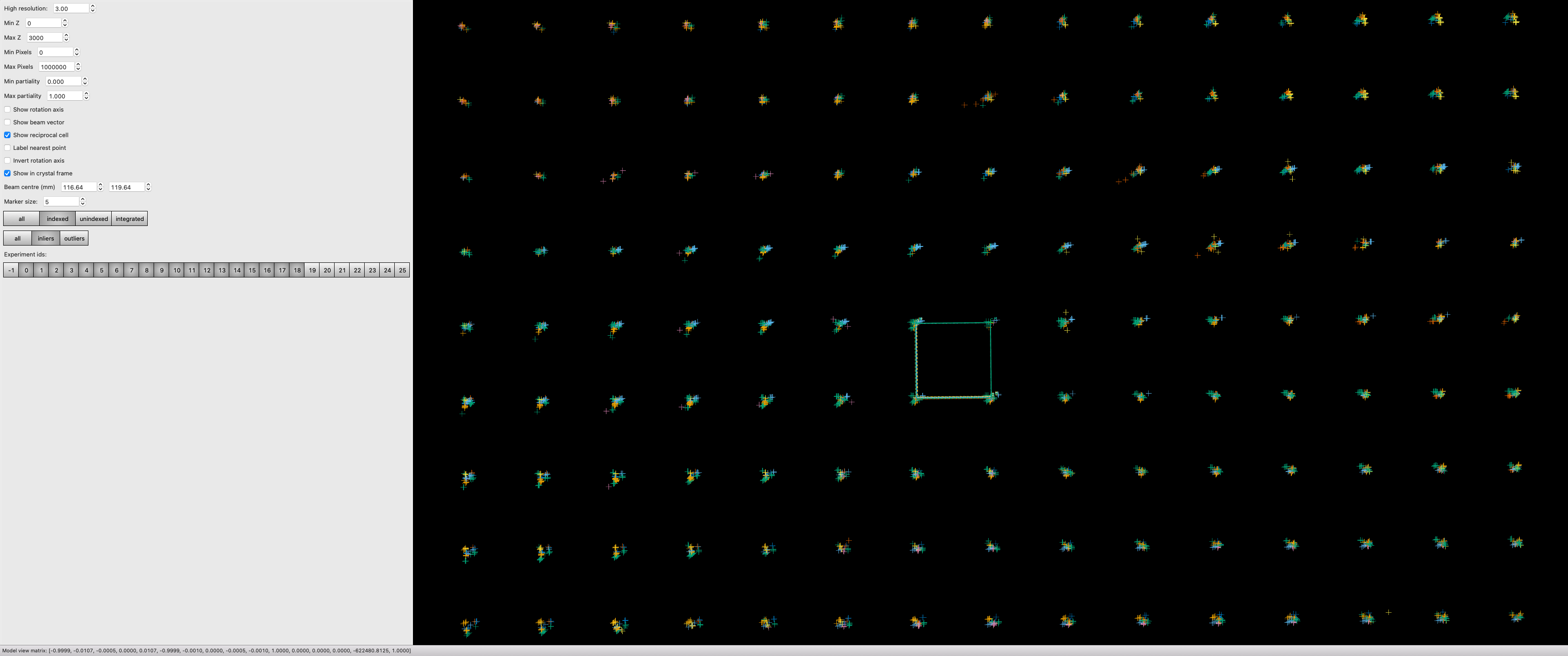
If you zoom in and switch on the reciprocal cells, this also allows you to actually see the Miller indices by counting from the origin outwards in multiples of the reciprocal cell:
Post Experiment Processing
Once all the data are processed you can use a tool from xia2 called
xia.multiplex - this will do many of the steps listed above and more, to
assess how well the data sets agree in a pairwise manner:
mplex $ xia2.multiplex ../sweep-*/integrated.* min_completeness=0.9
Now we can start asking some tricky questions about the best subsets
of data to use for the next steps in your data analysis. This command
will keep all the clusters which are >= 90% complete, then scale and
merge the data for each of those clusters to allow direct comparison -
here inspection of the generated xia2.multiplex.html is critical. There is
a lot of information in there so worth paying attention to. Here we go over
some of the commonly useful sections of the report.
Preferential Orientation
One risk with in situ data collection is that the samples can grow with a particular crystallographic axis, perpendicular to the plate. This in turn means that small rotations with the plate perpendicular to the beam will repeatedly record the same small volumes of reciprocal space. This may be assessed by considering the distributions of the unit cell axes in reciprocal space - via a stereographic projection:
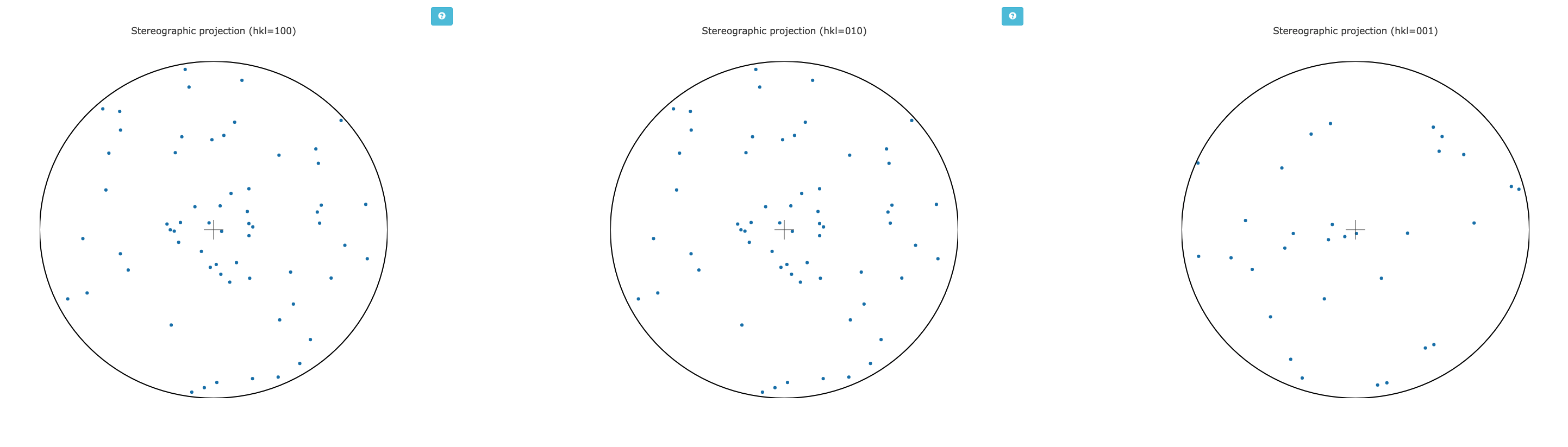
If all the dots are widely distributed around the circles - then there is no evidence of preferred orientation. If you have the dots all in the centre or all around the edge, then the axis is preferentially aligned with the beam or with the plate respectively, and you will need to consider carefully how to proceed with data collection.
Unit Cell Comparisons
The crystallographic unit cell can be used to give some hints of isomorphism, before intensity data are compared. If you have two distinct crystal forms they will be visible in these histograms:
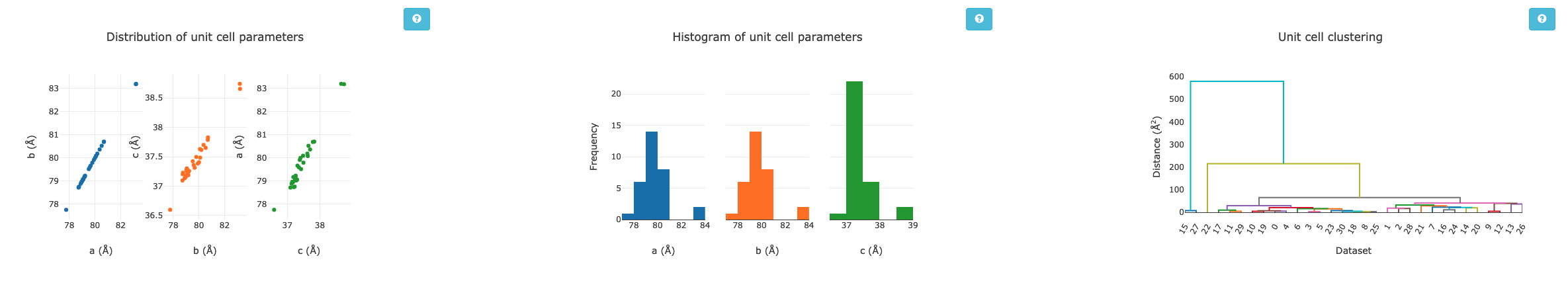
In this case, we have a reasonable spread of unit cells with two apparent outliers - with these data they are most likely to be better identified by intensity comparisons, but in some cases the unit cell information could provide more useful insight.
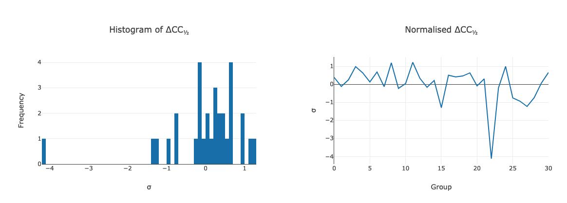
Delta CC-half
This is possibly more useful than specific unit cell outliers - showing the
data which add or detract from the data set as a whole - this was already
touched upon in the discussion above. The data may be excluded by taking the
data from the scaled full cluster, and passing this in to dials.scale with
the exclude_datasets= option.
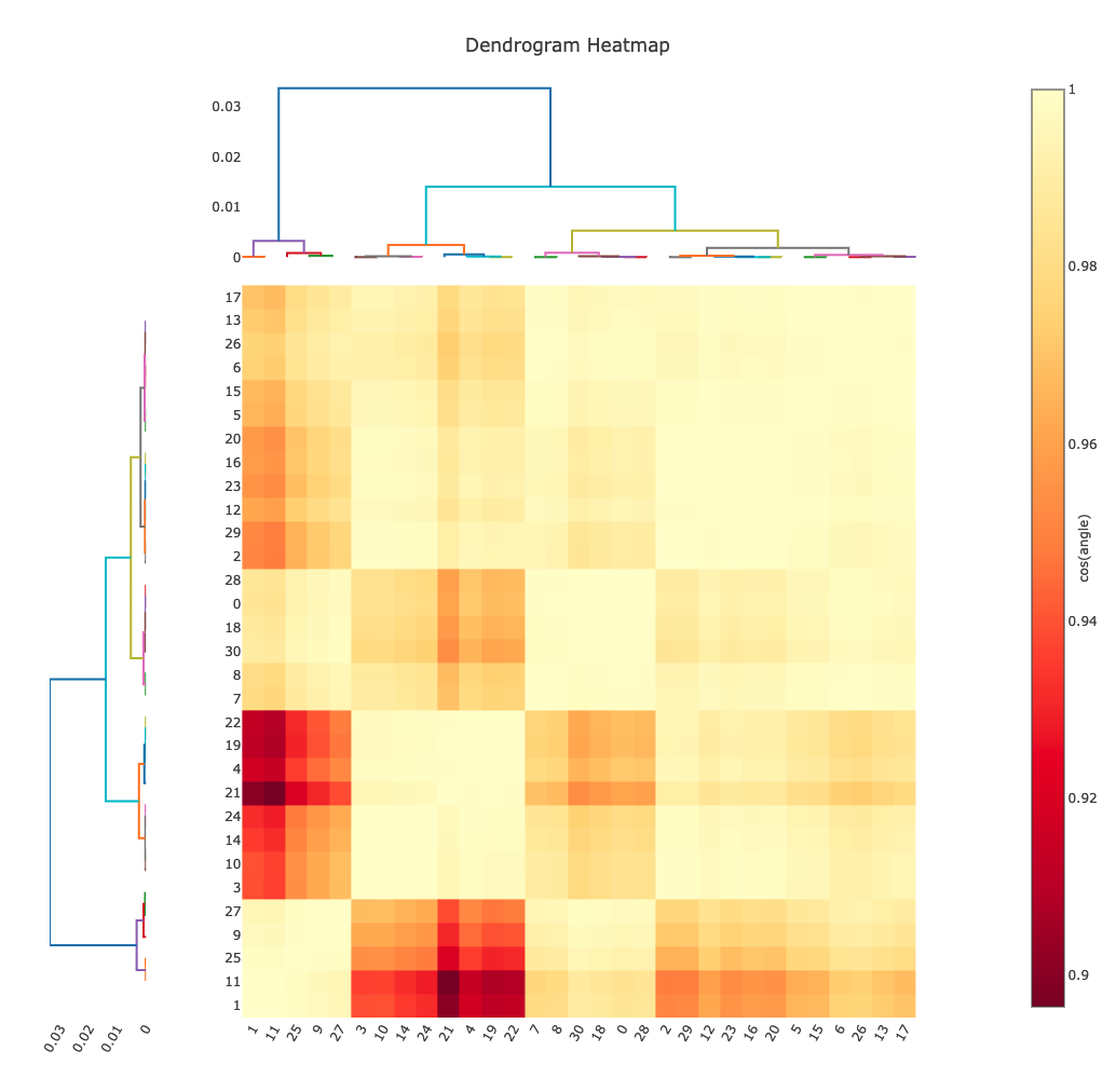
Intensity Clustering
Here we are assessing the correlation between pairs of data sets - if these are relatively complete this can very rapidly give you an idea of which data should be merged. Here we see the so-called “cos angle” clustering which is an assessment of the similarity independent of the strength of the individual data sets, and there are (depending on your criteria) maybe three or four distinct clusters. It is these clusters which are then considered in the next section.
Cluster Comparisons
This is where we can really start to inspect the details of relations between
data sets: the possible clusters that have been identified by
xia2.multiplex, with completeness >= 90%, can be compared by their overall
and per-resolution-shell merging statistics:
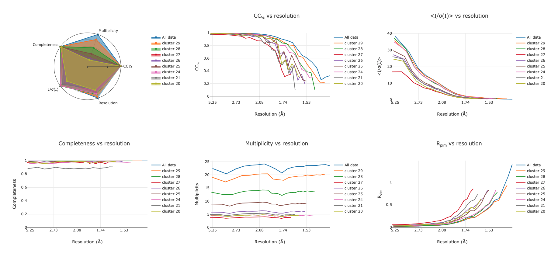
These allow you to select the best cluster according to your own criteria, before proceeding.
For each cluster here, you will find a subdirectory inside the folder you ran
xia2.multiplex. This subdirectory containing all of the analysis output and
the final scaled data for that cluster, scaled independently of the other
clusters. For example:
mplex $ cd cluster_20
cluster_20 $ ls
27_dials.two_theta_refine.cif       dials.estimate_resolution.log
27_dials.two_theta_refine.json      dials.scale.log
27_dials.two_theta_refine.log       dials.two_theta_refine.log
27_dials.two_theta_refine.mmcif     models.expt
27_dials.two_theta_refine.p4p       multiplicities_h_0.json
27_dials.two_theta_refine_2theta.png    multiplicities_h_0.png
27_refined_cell.expt            multiplicities_k_0.json
28_dials.scale.log          multiplicities_k_0.png
28_scaled.expt              multiplicities_l_0.json
28_scaled.mtz               multiplicities_l_0.png
28_scaled.refl              observations.refl
28_scaled_unmerged.mtz          scaled.expt
28_scaling.html             scaled.mtz
29_dials.estimate_resolution.html   scaled.refl
29_dials.estimate_resolution.json   scaled_unmerged.mtz
29_dials.estimate_resolution.log
contains everything you would need to take forward for that cluster,
allowing you to evaluate the success of processing for each downstream
step. The merging statistics for every cluster are also highlighted in
the tabs of the output in xia2.multiplex.html.