
Please click here to go to the tutorial for DIALS 2.2.
Multi-crystal analysis with DIALS and BLEND: individual vs joint refinement
Introduction
BLEND is a CCP4 program for analysis of multiple data sets. It attempts to identify isomorphous clusters that may be scaled and merged together to form a more complete multi-crystal dataset. Clustering in blend is based on the refined cell parameters from integration, so it is important that these are determined accurately. Unfortunately, for narrow wedges of data (where BLEND is most useful) cell refinement may be complicated by issues such as the high correlation between e.g. the detector distance and the cell volume.
One solution is to fix detector parameters during cell refinement so that the detector is the same for every dataset processed. However, this is only feasible if an accurate detector model is determined ahead of time, which might require the use of a well-diffracting sacrificial crystal. If we only have the narrow wedges of data available then it is more complicated to determine what the best detector model would be to fix.
If we can make the assumption that the beam and detector did not move during and between all of the datasets we collected then we can use DIALS joint refinement to refine all of the crystal cells at the same time, simultaneously with shared detector and beam models.
In this tutorial, we will attempt to do that for 73 sequences of data collected from crystals of TehA, a well-diffracting integral membrane protein measured using in situ diffraction from crystallisation plates at room temperature. Each sequence provides between 4 and 10 degrees of data.
This tutorial is relatively advanced in that it requires high level scripting of the DIALS command line programs, however candidate scripts are provided and the tutorial will hopefully be easy enough to follow.
Individual processing
We start with a directory full of images. It is easy enough to figure out
which files belong with which sequence from the filename templates, however note
that the pattern between templates is not totally consistent. Most of the sequences
start with the prefix xtal, but some have just xta. One way of
getting around this annoyance would be to use the fact that each dataset has
a single *.log file associated with it and identify the different
datasets that way. However, we would prefer to come up with a protocol that
would work more generally, not just for the TehA data. Happily we can just
let DIALS figure it out for us:
dials.import /path/to/TehA/*.cbf

The following parameters have been modified:

input {
  experiments = <image files>
}

--------------------------------------------------------------------------------
  format: <class 'dxtbx.format.FormatCBFMiniPilatus.FormatCBFMiniPilatus'>
  num images: 2711
  sequences:
    still:    0
    sweep:    73
  num stills: 0
--------------------------------------------------------------------------------
Writing experiments to imported.expt
With a single command we have determined that there are 73 individual sequences comprising 2711 total images. Running the following command will give us information about each one of these datasets:
dials.show imported.expt
That was a smooth start, but now things get abruptly more difficult. Before we perform the joint analysis, we want to do the individual analysis to compare to. This will also give us intermediate files so that we don’t have to start from scratch when setting up the joint refinement job. Essentially we just want to run a sequence of DIALS commands to process each recorded sequence. However we can’t (currently) split the experimentlist into individual sequences with a single command. We will have to start again with dials.import for each sequence individually - but we really don’t want to run this manually 73 times.
The solution is to write a script that will take the imported.expt as
input, extract the filename templates, and run the same processing commands
for each dataset. This script could be written in BASH, tcsh, perl,
ruby - whatever you feel most comfortable with. However here we will use Python,
or more specifically dials.python because we will take advantage of
features in the cctbx to make it easy to write scripts that take advantage
of parallel execution.
Also we would like to read imported.expt with the DIALS API rather than
extracting the sequence templates using something like grep.
The script we used to do this is reproduced below. You can copy this into a file,
save it as process_TehA.py and then run it as follows:
time dials.python process_TehA.py imported.expt
On a Linux desktop with a Core i7 CPU running at 3.07GHz the script took about 8
minutes to run (though file i/o is a significant factor)
and successfully processed 58 datasets. If time is short, you
might like to start running it now before reading the description of what the
script does. If time is really short then try uncommenting the line
tasklist = tasklist[0:35] to reduce the number of datasets processed.
#!/bin/env dials.python
import os
import sys
from libtbx import easy_run, easy_mp, Auto
from dxtbx.serialize import load


def process_sequence(task):
  """Process a single sequence of data. The parameter 'task' will be a
  tuple, the first element of which is an integer job number and the
  second is the filename template of the images to process"""

  num = task[0]
  template = task[1]

  # create directory
  newdir = os.getcwd()+"/sequence_%02d" % num
  os.mkdir(newdir)
  os.chdir(newdir)
  cmd = "dials.import template={0}".format(template)
  easy_run.fully_buffered(command=cmd)
  easy_run.fully_buffered(command="dials.find_spots imported.expt")

  # initial indexing in P 1
  cmd = "dials.index imported.expt strong.refl " +\
    "output.experiments=P1_models.expt"
  easy_run.fully_buffered(command=cmd)
  if not os.path.isfile("P1_models.expt"):
    print "Job %02d failed in initial indexing" % num
    return

  # bootstrap from the refined P 1 cell
  cmd = "dials.index P1_models.expt strong.refl space_group='H 3'"
  easy_run.fully_buffered(command=cmd)
  if not os.path.isfile("indexed.expt"):
    print "Job %02d failed in indexing" % num
    return

  # static model refinement
  cmd = "dials.refine indexed.expt indexed.refl scan_varying=false " + \
    "outlier.algorithm=tukey"
  easy_run.fully_buffered(command=cmd)
  if not os.path.isfile("refined.expt"):
    print "Job %02d failed in refinement" % num
    return

  # WARNING! Fast and dirty integration.
  # Do not use the result for scaling/merging!
  cmd = "dials.integrate refined.expt indexed.refl " + \
    "profile.fitting=False prediction.d_min=7.0 prediction.d_max=8.1"
  easy_run.fully_buffered(command=cmd)
  if not os.path.isfile("integrated.refl"):
    print "Job %02d failed during integration" % num
    return

  # create MTZ
  cmd = "dials.export refined.expt integrated.refl " +\
    "intensity=sum mtz.hklout=integrated.mtz"
  easy_run.fully_buffered(command=cmd)
  if not os.path.isfile("integrated.mtz"):
    print "Job %02d failed during MTZ export" % num
    return

  # if we got this far, return the path to the MTZ
  return "sequence_%02d/integrated.mtz" % num

if __name__ == "__main__":

  if len(sys.argv) != 2:
    sys.exit("Usage: dials.python process_TehA.py imported.expt")

  expt_path = os.path.abspath(sys.argv[1])
  experiments = load.experiment_list(expt_path, check_format=False)
  templates = [i.get_template() for i in experiments.imagesets()]
  tasklist = list(enumerate(sorted(templates)))

  if not tasklist:
    sys.exit("No images found!")

  # uncomment the following line if short on time!
  #tasklist = tasklist[0:35]

  nproc = easy_mp.get_processes(Auto)

  print "Attempting to process the following datasets, with {} processes".format(nproc)
  for task in tasklist:
    print "%d: %s" % task

  results = easy_mp.parallel_map(
    func=process_sequence,
    iterable=tasklist,
    processes=nproc,
    preserve_order=True,
  )

  good_results = [e for e in results if e is not None]
  print "Successfully created the following MTZs:"
  for result in good_results:
    print result
We will now describe what is in this script. The first lines are
just imports to bring in modules from the Python standard library as well as
easy_run and easy_mp from libtbx (part of cctbx),
serlialize.load from dxtbx to read in the ExperimentList.
Following that is a definition for the function
process_sequence which will perform all the steps required to process one
dataset from images to unmerged MTZ. The code block under:
if __name__ == "__main__":
are the lines that are executed when the script starts. First we check that the
script has been passed a path to an experiments file. We then extract the 73 sequences
from this into a list, then get the filename templates from each element in the
list. We associate each of these templates with a number to form a list of
‘tasks’ to pass into process_sequence, but instead
of doing this in serial we can use easy_mp to run in parallel. This will
be okay because inside process_sequence, we ensure that all results are
written into a new directory. First we use a facility of the easy_mp
module to determine the number of processes to run in parallel and then we submit
the job with parallel_map.
The commands that are inside the function are usual dials commands,
familiar from other tutorials. There are a couple of interesting points
to note though. We know that the correct space group is H 3, but it turns out
that if we ask dials.index to find an H 3 cell right from the start
then many of the sequences fail to index. This is simply because the initial models
contained in imported.expt are too poor to locate a cell with the
symmetry constraints. However, for many of the sequences the indexing program will
refine the P 1 solution to the correct cell. For this reason we first run
indexing in P 1:
dials.index imported.expt strong.refl output.experiments=P1_models.expt
and then we feed the refined P1_models.expt back into
dials.index specifying the correct symmetry:
dials.index P1_models.expt strong.refl space_group='H 3'
When dials.index is passed a models.expt containing
a crystal model rather than just a imported.expt then it automatically
uses a known_orientation indexer, which avoids doing the basis vector
search again. It uses the basis of the refined P 1 cell and just assigns
indices under the assumption of H 3 symmetry. The symmetry constraints are
then enforced during the refinement steps carried out by dials.index.
This procedure gives us a greater success rate of indexing in H 3, and required
no manual intervention.
Following indexing we do scan-static cell refinement:
dials.refine indexed.expt indexed.refl scan_varying=false outlier.algorithm=tukey
Outlier rejection was switched on in an attempt to avoid any zingers or other
errant spots from affecting our refined cells. Without analysing the data closer
it is not clear whether there are any particularly bad outliers here. We could repeat
the whole analysis with this switched off if we want to investigate more closely,
or look through all the dials.refine.log files to see results of the
outlier rejection step.
We don’t bother with the time-consuming step of scan-varying refinement, because it is the scan-static cell that will be written into the MTZ header. Scan- varying refinement would give us better models for integration but as we will only be running blend in ‘analysis’ mode we are in the unusual situation of not actually caring what the intensities are. In this case, the MTZ file is just a carrier for the globally refined unit cell!
Following refinement we integrate the data in a very quick and dirty way, simply to get an MTZ file as fast as possible. This is a terrible way to integrate data usually!:
dials.integrate refined.expt indexed.refl profile.fitting=False prediction.d_min=7.0 prediction.d_max=8.1
The profile.fitting=False option ensures we only do summation integration,
no profile fitting, while the prediction.dmin=7.0 and
prediction.dmax=8.1 options only integrate data between 7.0 and 8.1 Angstroms.
As a result few reflections will be integrated. The MTZ file here is just
being used as a carrier of the cell information into blend. By restricting the
resolution range this way we are making it obvious that the content of the file
is useless for any other purpose.
Warning
Do not use the data produced by this script for scaling and merging. More careful processing should be done first!
Finally we use dials.export to create an MTZ file:
dials.export refined.expt integrated.refl intensity=sum mtz.hklout=integrated.mtz
After each of these major steps we check whether the last command ran successfully
by checking for the existence of an expected output file. If the file does not
exist we make no effort to rescue the dataset, we just return early from the
process_sequence function, freeing up a process so that
parallel_map can start up the next.
Here is the output of a run of the script:
Attempting to process the following datasets, with 5 processes
0: /joint-refinement-img/xta30_1_####.cbf
1: /joint-refinement-img/xta31_1_####.cbf

...

71: /joint-refinement-img/xtal7_1_####.cbf
72: /joint-refinement-img/xtal8_1_####.cbf
Job 06 failed in initial indexing
Job 05 failed during integration
Job 07 failed during integration
Job 10 failed during integration
Job 15 failed during integration
Job 18 failed during integration
Job 30 failed during integration
Job 34 failed during integration
Job 37 failed in initial indexing
Job 36 failed during integration
Job 52 failed in initial indexing
Job 51 failed during integration
Job 49 failed during integration
Job 56 failed during integration
Job 72 failed during integration
Successfully created the following MTZs:
sequence_00/integrated.mtz
sequence_01/integrated.mtz
sequence_02/integrated.mtz
sequence_03/integrated.mtz
sequence_04/integrated.mtz
sequence_08/integrated.mtz
sequence_09/integrated.mtz
sequence_11/integrated.mtz
sequence_12/integrated.mtz
sequence_13/integrated.mtz
sequence_14/integrated.mtz
sequence_16/integrated.mtz
sequence_17/integrated.mtz
sequence_19/integrated.mtz
sequence_20/integrated.mtz
sequence_21/integrated.mtz
sequence_22/integrated.mtz
sequence_23/integrated.mtz
sequence_24/integrated.mtz
sequence_25/integrated.mtz
sequence_26/integrated.mtz
sequence_27/integrated.mtz
sequence_28/integrated.mtz
sequence_29/integrated.mtz
sequence_31/integrated.mtz
sequence_32/integrated.mtz
sequence_33/integrated.mtz
sequence_35/integrated.mtz
sequence_38/integrated.mtz
sequence_39/integrated.mtz
sequence_40/integrated.mtz
sequence_41/integrated.mtz
sequence_42/integrated.mtz
sequence_43/integrated.mtz
sequence_44/integrated.mtz
sequence_45/integrated.mtz
sequence_46/integrated.mtz
sequence_47/integrated.mtz
sequence_48/integrated.mtz
sequence_50/integrated.mtz
sequence_53/integrated.mtz
sequence_54/integrated.mtz
sequence_55/integrated.mtz
sequence_57/integrated.mtz
sequence_58/integrated.mtz
sequence_59/integrated.mtz
sequence_60/integrated.mtz
sequence_61/integrated.mtz
sequence_62/integrated.mtz
sequence_63/integrated.mtz
sequence_64/integrated.mtz
sequence_65/integrated.mtz
sequence_66/integrated.mtz
sequence_67/integrated.mtz
sequence_68/integrated.mtz
sequence_69/integrated.mtz
sequence_70/integrated.mtz
sequence_71/integrated.mtz

real  9m56.401s
user  29m36.650s
sys     8m3.996s
Analysis of individually processed datasets
The paths to integrated.mtz files can be copied directly into a file,
say individual_mtzs.dat, and passed to BLEND for analysis:
echo "END" | blend -a individual_mtzs.dat
The dendrogram resulting from clustering is shown here:
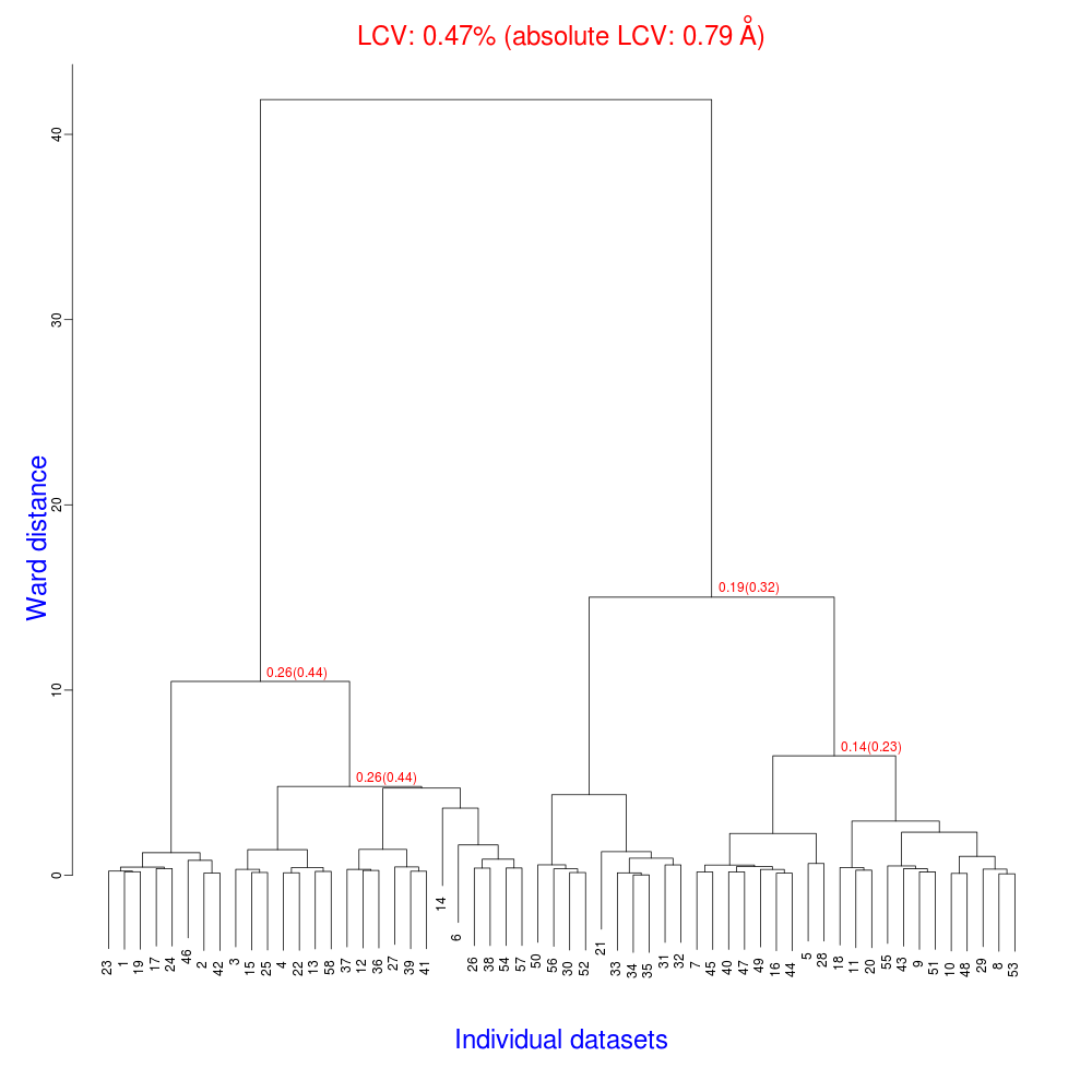
As we can see, the linear cell variation is less than 1%, with an absolute
value of 0.79 Angstroms, indicating good isomorphism amongst the datasets.
If any extreme outliers had been shown by the plot, one can inspect the
file FINAL_list_of_files.dat to see which sequence the blend numbering
relates to. These files could then be removed from individual_mtzs.dat
before rerunning BLEND.
Joint refinement
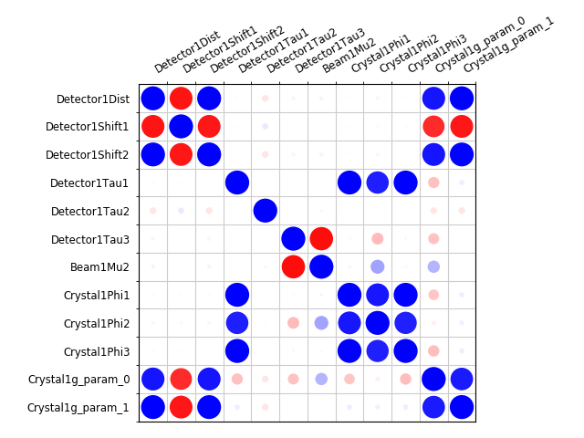
Now that we have done the BLEND analysis for individually processed datasets, we would like to do joint refinement of the crystals to reduce correlations between the detector or beam parameters with individual crystals. As motivation we may look at these correlations for one of these datasets. For example:
cd sequence_00
dials.refine indexed.expt indexed.refl scan_varying=false \
  track_parameter_correlation=true correlation_plot.filename=corrplot.png
cd ..
The new file sequence_00/corrplot_X.png shows correlations between parameters
refined with this single 8 degree dataset (see also correlations in Y and Phi).
Clearly parameters like the detector distance and the crystal metrical matrix
parameters are highly correlated.
Although the DIALS toolkit has a sophisticated mechanism for modelling
multi-experiment data, the user interface for handling such data is somewhat
limited. In order to do joint refinement of the sequences we need to combine them
into a single multi-experiment combined.expt and corresponding
combined.refl. Whilst doing this we want to reduce the separate
detector, beam and goniometer models for each experiment into a single shared
model of each type. The program dials.combine_experiments can
be used for this, but first we have to prepare an input file with a text editor
listing the individual sequences in order. We can use
individual_mtzs.dat as a template to start with. In our case the final
file looks like this:
input {
  experiments = sequence_00/refined.expt
  experiments = sequence_01/refined.expt
  experiments = sequence_02/refined.expt
  experiments = sequence_03/refined.expt
  experiments = sequence_04/refined.expt
  experiments = sequence_08/refined.expt
  experiments = sequence_09/refined.expt
  experiments = sequence_11/refined.expt
  experiments = sequence_12/refined.expt
  experiments = sequence_13/refined.expt
  experiments = sequence_14/refined.expt
  experiments = sequence_16/refined.expt
  experiments = sequence_17/refined.expt
  experiments = sequence_19/refined.expt
  experiments = sequence_20/refined.expt
  experiments = sequence_21/refined.expt
  experiments = sequence_22/refined.expt
  experiments = sequence_23/refined.expt
  experiments = sequence_24/refined.expt
  experiments = sequence_25/refined.expt
  experiments = sequence_26/refined.expt
  experiments = sequence_27/refined.expt
  experiments = sequence_28/refined.expt
  experiments = sequence_29/refined.expt
  experiments = sequence_31/refined.expt
  experiments = sequence_32/refined.expt
  experiments = sequence_33/refined.expt
  experiments = sequence_35/refined.expt
  experiments = sequence_38/refined.expt
  experiments = sequence_39/refined.expt
  experiments = sequence_40/refined.expt
  experiments = sequence_41/refined.expt
  experiments = sequence_42/refined.expt
  experiments = sequence_43/refined.expt
  experiments = sequence_44/refined.expt
  experiments = sequence_45/refined.expt
  experiments = sequence_46/refined.expt
  experiments = sequence_47/refined.expt
  experiments = sequence_48/refined.expt
  experiments = sequence_50/refined.expt
  experiments = sequence_53/refined.expt
  experiments = sequence_54/refined.expt
  experiments = sequence_55/refined.expt
  experiments = sequence_57/refined.expt
  experiments = sequence_58/refined.expt
  experiments = sequence_59/refined.expt
  experiments = sequence_60/refined.expt
  experiments = sequence_61/refined.expt
  experiments = sequence_62/refined.expt
  experiments = sequence_63/refined.expt
  experiments = sequence_64/refined.expt
  experiments = sequence_65/refined.expt
  experiments = sequence_66/refined.expt
  experiments = sequence_67/refined.expt
  experiments = sequence_68/refined.expt
  experiments = sequence_69/refined.expt
  experiments = sequence_70/refined.expt
  experiments = sequence_71/refined.expt
  reflections = sequence_00/indexed.refl
  reflections = sequence_01/indexed.refl
  reflections = sequence_02/indexed.refl
  reflections = sequence_03/indexed.refl
  reflections = sequence_04/indexed.refl
  reflections = sequence_08/indexed.refl
  reflections = sequence_09/indexed.refl
  reflections = sequence_11/indexed.refl
  reflections = sequence_12/indexed.refl
  reflections = sequence_13/indexed.refl
  reflections = sequence_14/indexed.refl
  reflections = sequence_16/indexed.refl
  reflections = sequence_17/indexed.refl
  reflections = sequence_19/indexed.refl
  reflections = sequence_20/indexed.refl
  reflections = sequence_21/indexed.refl
  reflections = sequence_22/indexed.refl
  reflections = sequence_23/indexed.refl
  reflections = sequence_24/indexed.refl
  reflections = sequence_25/indexed.refl
  reflections = sequence_26/indexed.refl
  reflections = sequence_27/indexed.refl
  reflections = sequence_28/indexed.refl
  reflections = sequence_29/indexed.refl
  reflections = sequence_31/indexed.refl
  reflections = sequence_32/indexed.refl
  reflections = sequence_33/indexed.refl
  reflections = sequence_35/indexed.refl
  reflections = sequence_38/indexed.refl
  reflections = sequence_39/indexed.refl
  reflections = sequence_40/indexed.refl
  reflections = sequence_41/indexed.refl
  reflections = sequence_42/indexed.refl
  reflections = sequence_43/indexed.refl
  reflections = sequence_44/indexed.refl
  reflections = sequence_45/indexed.refl
  reflections = sequence_46/indexed.refl
  reflections = sequence_47/indexed.refl
  reflections = sequence_48/indexed.refl
  reflections = sequence_50/indexed.refl
  reflections = sequence_53/indexed.refl
  reflections = sequence_54/indexed.refl
  reflections = sequence_55/indexed.refl
  reflections = sequence_57/indexed.refl
  reflections = sequence_58/indexed.refl
  reflections = sequence_59/indexed.refl
  reflections = sequence_60/indexed.refl
  reflections = sequence_61/indexed.refl
  reflections = sequence_62/indexed.refl
  reflections = sequence_63/indexed.refl
  reflections = sequence_64/indexed.refl
  reflections = sequence_65/indexed.refl
  reflections = sequence_66/indexed.refl
  reflections = sequence_67/indexed.refl
  reflections = sequence_68/indexed.refl
  reflections = sequence_69/indexed.refl
  reflections = sequence_70/indexed.refl
  reflections = sequence_71/indexed.refl
}
We called this file experiments_and_reflections.phil then run
dials.combine_experiments like this:
dials.combine_experiments experiments_and_reflections.phil \
  reference_from_experiment.beam=0 \
  reference_from_experiment.goniometer=0 \
  reference_from_experiment.detector=0 \
  compare_models=False
The reference_from_experiment options tell the program to replace all
beam, goniometer and detector models in the input experiments with those
models taken from the first experiment, i.e. experiment ‘0’ using 0-based
indexing. If you run without compare_models=False, you’ll see that the beam
models are not similar enough to pass the tolerance tests in combine_experiments.
The output lists the number of reflections in each sequence contributing
to the final combined.refl:
--------------------------------------
| Experiment | Number of reflections |
--------------------------------------
| 0          | 1471                  |
| 1          | 1464                  |
| 2          | 1232                  |
| 3          | 1381                  |
| 4          | 1588                  |
| 5          | 616                   |
| 6          | 1642                  |
| 7          | 1083                  |
| 8          | 1210                  |
| 9          | 1000                  |
| 10         | 1529                  |
| 11         | 1430                  |
| 12         | 1261                  |
| 13         | 1587                  |
| 14         | 1727                  |
| 15         | 1358                  |
| 16         | 1049                  |
| 17         | 1830                  |
| 18         | 1477                  |
| 19         | 2033                  |
| 20         | 1308                  |
| 21         | 1856                  |
| 22         | 1830                  |
| 23         | 1654                  |
| 24         | 1048                  |
| 25         | 1695                  |
| 26         | 2398                  |
| 27         | 2173                  |
| 28         | 2869                  |
| 29         | 3181                  |
| 30         | 2810                  |
| 31         | 1563                  |
| 32         | 3508                  |
| 33         | 2985                  |
| 34         | 2526                  |
| 35         | 2453                  |
| 36         | 1738                  |
| 37         | 1152                  |
| 38         | 981                   |
| 39         | 1336                  |
| 40         | 1331                  |
| 41         | 641                   |
| 42         | 1052                  |
| 43         | 1364                  |
| 44         | 2114                  |
| 45         | 2063                  |
| 46         | 2139                  |
| 47         | 1570                  |
| 48         | 2334                  |
| 49         | 1645                  |
| 50         | 2499                  |
| 51         | 2227                  |
| 52         | 971                   |
| 53         | 1130                  |
| 54         | 2376                  |
| 55         | 1211                  |
| 56         | 1190                  |
| 57         | 652                   |
--------------------------------------
Saving combined experiments to combined.expt
Saving combined reflections to combined.refl
We may also inspect the contents of combined.expt, by using
dials.show, for example:
dials.show combined.expt
Useful though this is, it is clear how this could become unwieldy as the number of experiments increases. Work on better interfaces to multi-crystal (or generally, multi-experiment) data is ongoing within the DIALS project. Suggestions are always welcome!
Now we have the joint experiments and reflections files we can run our multi- crystal refinement job:
dials.refine combined.expt combined.refl \
  scan_varying=false outlier.algorithm=tukey
The following parameters have been modified:

refinement {
  parameterisation {
    scan_varying = False
  }
  reflections {
    outlier {
      algorithm = null auto mcd *tukey sauter_poon
    }
  }
}
input {
  experiments = combined.expt
  reflections = combined.refl
}

Configuring refiner

Summary statistics for 96848 observations matched to predictions:
--------------------------------------------------------------------
|                   | Min    | Q1      | Med      | Q3     | Max   |
--------------------------------------------------------------------
| Xc - Xo (mm)      | -9.637 | -0.8559 | -0.04029 | 0.8264 | 13.31 |
| Yc - Yo (mm)      | -27.99 | -0.5649 | -0.02585 | 0.4819 | 27.1  |
| Phic - Phio (deg) | -37.46 | -0.1734 | 0.001499 | 0.1756 | 39.32 |
| X weights         | 232.3  | 359.5   | 378.5    | 392.9  | 405.6 |
| Y weights         | 246.2  | 390.2   | 399      | 403.2  | 405.6 |
| Phi weights       | 262.1  | 299.8   | 300      | 300    | 300   |
--------------------------------------------------------------------

Detecting centroid outliers using the Tukey algorithm
9352 reflections have been flagged as outliers

Summary statistics for 87496 observations matched to predictions:
--------------------------------------------------------------------
|                   | Min    | Q1      | Med      | Q3     | Max   |
--------------------------------------------------------------------
| Xc - Xo (mm)      | -9.637 | -0.89   | -0.02594 | 0.8807 | 13.31 |
| Yc - Yo (mm)      | -11.78 | -0.5064 | -0.02297 | 0.4352 | 11.87 |
| Phic - Phio (deg) | -8.19  | -0.1399 | 0.001485 | 0.1429 | 8.693 |
| X weights         | 232.3  | 359.3   | 378.3    | 392.6  | 405.6 |
| Y weights         | 246.2  | 390.6   | 399.1    | 403.2  | 405.6 |
| Phi weights       | 262.1  | 300     | 300      | 300    | 300   |
--------------------------------------------------------------------

There are 297 parameters to refine against 87496 reflections in 3 dimensions
Performing refinement of 58 Experiments...

Refinement steps:
-----------------------------------------------
| Step | Nref  | RMSD_X  | RMSD_Y  | RMSD_Phi |
|      |       | (mm)    | (mm)    | (deg)    |
-----------------------------------------------
| 0    | 87496 | 1.6408  | 1.1569  | 0.79118  |
| 1    | 87496 | 1.0856  | 0.83106 | 0.52798  |
| 2    | 87496 | 0.91236 | 0.7085  | 0.50131  |
| 3    | 87496 | 0.70048 | 0.54736 | 0.46902  |
| 4    | 87496 | 0.46951 | 0.36137 | 0.40123  |
| 5    | 87496 | 0.29632 | 0.21747 | 0.28785  |
| 6    | 87496 | 0.20347 | 0.15376 | 0.17079  |
| 7    | 87496 | 0.16762 | 0.13534 | 0.11626  |
| 8    | 87496 | 0.16252 | 0.13282 | 0.10889  |
| 9    | 87496 | 0.16223 | 0.13265 | 0.1086   |
| 10   | 87496 | 0.16213 | 0.13258 | 0.1086   |
| 11   | 87496 | 0.16204 | 0.13254 | 0.10869  |
| 12   | 87496 | 0.162   | 0.13252 | 0.10877  |
| 13   | 87496 | 0.16199 | 0.13252 | 0.10879  |
| 14   | 87496 | 0.16199 | 0.13252 | 0.10879  |
-----------------------------------------------
RMSD no longer decreasing

RMSDs by experiment:
---------------------------------------------
| Exp | Nref | RMSD_X  | RMSD_Y  | RMSD_Z   |
| id  |      | (px)    | (px)    | (images) |
---------------------------------------------
| 0   | 1438 | 0.55006 | 0.36386 | 0.39245  |
| 1   | 1377 | 0.60375 | 0.35395 | 0.37074  |
| 2   | 1046 | 0.81377 | 0.55378 | 0.74578  |
| 3   | 1042 | 0.71331 | 0.50699 | 0.29662  |
| 4   | 1430 | 1.7057  | 2.0768  | 0.70272  |
| 5   | 562  | 0.76136 | 0.54465 | 0.444    |
| 6   | 1473 | 0.91579 | 1.2153  | 0.38596  |
| 7   | 1033 | 0.50161 | 0.37586 | 0.24255  |
| 8   | 1097 | 0.49387 | 0.35304 | 0.27443  |
| 9   | 871  | 0.8339  | 0.58238 | 0.27862  |
| 10  | 1462 | 0.51758 | 0.29764 | 0.26121  |
| 11  | 1297 | 1.0496  | 1.0934  | 0.62916  |
| 12  | 1060 | 0.56529 | 0.41568 | 0.35943  |
| 13  | 1508 | 0.52573 | 0.34911 | 0.2364   |
| 14  | 1581 | 0.64887 | 0.3499  | 0.27855  |
| 15  | 1142 | 1.3555  | 1.0016  | 0.81589  |
| 16  | 987  | 0.57376 | 0.46291 | 0.30225  |
| 17  | 1642 | 0.68198 | 0.55891 | 0.48053  |
| 18  | 1334 | 0.62128 | 0.55331 | 0.34444  |
| 19  | 1814 | 0.97204 | 0.80027 | 0.48625  |
| 20  | 1172 | 0.82146 | 0.47213 | 0.41469  |
| 21  | 1696 | 0.65721 | 0.34464 | 0.28293  |
| 22  | 1700 | 0.59074 | 0.37139 | 0.28981  |
| 23  | 1472 | 0.72438 | 0.69007 | 0.39294  |
| 24  | 886  | 0.81814 | 0.64633 | 0.39922  |
| 25  | 1413 | 1.5227  | 1.839   | 0.90807  |
| 26  | 2374 | 0.52255 | 0.2912  | 0.24541  |
| 27  | 1998 | 0.494   | 0.29952 | 0.23895  |
| 28  | 2620 | 0.5181  | 0.30387 | 0.25139  |
| 29  | 2928 | 0.51628 | 0.29307 | 0.27191  |
| 30  | 2510 | 0.51078 | 0.3342  | 0.29667  |
| 31  | 1334 | 0.68191 | 0.38606 | 0.2856   |
| 32  | 3240 | 0.80437 | 0.50846 | 0.5801   |
| 33  | 2330 | 1.5782  | 1.0468  | 0.59145  |
| 34  | 2409 | 0.64632 | 0.28538 | 0.26755  |
| 35  | 2226 | 1.944   | 1.6115  | 0.86348  |
| 36  | 1551 | 0.91913 | 0.90458 | 0.64259  |
| 37  | 1047 | 0.75458 | 0.54531 | 0.30649  |
| 38  | 742  | 1.6069  | 1.0673  | 1.3176   |
| 39  | 1205 | 1.2038  | 0.94187 | 1.0289   |
| 40  | 1200 | 1.3346  | 0.98056 | 0.46257  |
| 41  | 502  | 1.6651  | 1.159   | 1.7142   |
| 42  | 939  | 2.2596  | 1.5491  | 2.0847   |
| 43  | 1105 | 1.1467  | 0.86945 | 1.0626   |
| 44  | 1929 | 0.55025 | 0.2708  | 0.25013  |
| 45  | 1786 | 0.60951 | 0.27533 | 0.27842  |
| 46  | 1738 | 0.56749 | 0.35204 | 0.33809  |
| 47  | 1454 | 0.53203 | 0.31578 | 0.27452  |
| 48  | 2016 | 1.1326  | 1.2978  | 0.59713  |
| 49  | 1481 | 0.97476 | 1.0774  | 0.32288  |
| 50  | 2412 | 0.54143 | 0.47678 | 0.25686  |
| 51  | 2005 | 1.0293  | 0.77775 | 0.46855  |
| 52  | 924  | 0.97306 | 0.64495 | 0.28243  |
| 53  | 1046 | 0.63827 | 0.42478 | 0.58041  |
| 54  | 2180 | 0.58521 | 0.32623 | 0.31898  |
| 55  | 1094 | 0.63002 | 0.40298 | 0.26934  |
| 56  | 1070 | 1.3311  | 1.0275  | 0.73719  |
| 57  | 566  | 2.3765  | 1.2727  | 0.78839  |
---------------------------------------------
Updating predictions for indexed reflections
Saving refined experiments to refined.expt
Saving reflections with updated predictions to refined.refl
The overall final RMSDs are 0.16 mm in X, 0.13 mm in Y and 0.11 degrees in \(\phi\). The RMSDs per experiment are also shown, which exhibit significant variation between datasets.
We can compare the RMSDs from individually refined experiments to those from
the joint experiments. For example, look at the RSMDs for experiment 1, in the
logfile sequence_01/dials.refine.log:
RMSDs by experiment:
---------------------------------------------
| Exp | Nref | RMSD_X  | RMSD_Y  | RMSD_Z   |
| id  |      | (px)    | (px)    | (images) |
---------------------------------------------
| 0   | 1422 | 0.54278 | 0.30358 | 0.2555   |
---------------------------------------------
Clearly allowing the detector and beam to refine only against this data lets the model better fit the observations, but is it a more accurate description of reality? Given that we know or can comfortably assume that the detector and beam did not move between data collections, then the constraints applied by joint refinement seem appropriate. The RMSDs for experiment 1 are not so much worse than from the individual refinement job. We are happy with this result and move on to re-integrating the data to create MTZs for BLEND.
It is worth noting that including/excluding outlier rejection can have a significant effect on the stability of the refinement (although not in this case). If issues are encountered processing your own data, try without outlier rejection to see if the result is improved.
Analysis of jointly refined datasets
We can run dials.integrate on the combined datafiles. We’ll do a ‘quick and dirty’ integration like before, to enable a fair comparison to be made for the BLEND results:
dials.integrate combined.refl refined.expt \
  prediction.d_min=7.0 prediction.d_max=8.1 \
  profile.fitting=False
This will integrate each dataset without profile fitting, using multiple processors, but only between 7.0 and 8.1 Angstrom to produce a quick result for the purpose of creating the MTZ files for BLEND. Next, we want to generate mtz files, however dials.export can only export one dataset at a time, so we will first need to separate the dataset into individual files:
dials.split_experiments integrated.refl integrated.expt
This will create a series of datafiles from
split_00.refl, split_00.expt up to
split_57.refl, split_57.expt.
To export the 58 datasets, we should write a script to avoid having to work manually. Currently, many DIALS programs such as dials.export can be imported into python scripts as functions to be called directly. Therefore the script we need is as follows:
#!/bin/env dials.python
import logging
from dxtbx.serialize import load
from dials.array_family import flex
from dials.util import log
from dials.command_line.export import phil_scope, export_mtz

logger = logging.getLogger("dials.command_line.export")

if __name__ == "__main__":

  log.config(logfile="export_all.log")

  params = phil_scope.extract()
  params.intensity = ["sum"]

  for i in range(0, 58):
      params.mtz.hklout = "integrated_%02d.mtz" % i
      logger.info("Attempting to export to %s", params.mtz.hklout)
      refl = flex.reflection_table.from_file("split_%02d.refl" % i)
      expts = load.experiment_list("split_%02d.expt" % i, check_format=False)
      export_mtz(params, expts, [refl])
This, if saved as joint_export.py, can be run as simply:
dials.python joint_export.py
This simple script has several key components. The ‘phil_scope’ contains the command-line program parameters, which we extract to a ‘params’ object for the export_mtz function call. We can override parameters in the params object, in this example we set the intensity type to export and set a new mtz filename for each iteration in the loop. We also need to provide a reflection table and experiment list for each dataset, which are loaded within the loop and passed to export_mtz. We also create a logger to capture any output from the export_mtz function, which we have to configure in the program. For this simple task, where we don’t need to take advantage of parallel processing, this script is sufficient.
As expected this creates all 58 MTZs for the jointly refined sequences without any
problem. We can copy the paths to these into a new file, say
joint_mtzs.dat, and run blend:
echo "END" | blend -a joint_mtzs.dat
The tree.png resulting from this is very interesting.
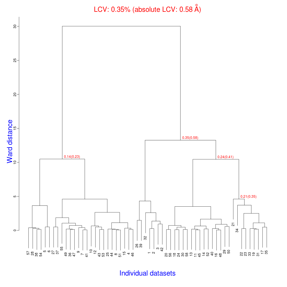
The LCV is now as low as 0.35% (aLCV 0.58 Angstroms). This indicates an even higher degree of isomorphism than detected during after individual processing. So although joint refinement leads to slightly higher RMSDs for each experiment (as we expected) the resulting unit cells are more similar. It is worth remembering that no restraints were applied between unit cells in refinement. Given that we know that the detector and beam did not move between the data collections we might like to think that the joint refinement analysis is a more accurate depiction of reality, and thus the unit cells are closer to the truth.
What to do next?
This has given us a good starting point for analysis with BLEND. However, because of the shortcuts we took with integration we are not yet ready to continue with BLEND’s synthesis mode. At this point we might assess where we are and try a few things:
Go back and fix datasets that didn’t index properly. We could edit our processing script to attempt
method=fft1dfor example if the 3D FFT indexing was unsuccessful.Integrate data properly for BLEND’s synthesis mode. We should remove the resolution limits and allow dials.integrate to do profile fitting as well as summation integration.
Acknowledgements
The TehA project and original BLEND analysis was performed by scientists at Diamond Light Source and the Membrane Protein Laboratory. We thank the following for access to the data: Danny Axford, Nien-Jen Hu, James Foadi, Hassanul Ghani Choudhury, So Iwata, Konstantinos Beis, Pierre Aller, Gwyndaf Evans & Yilmaz Alguel