
Please click here to go to the tutorial for DIALS 2.2.
Small-molecule data reduction tutorial
Introduction
While the conventional use of DIALS for small molecule data could be to run xia2, the interactive processing steps via the command line are relatively straightforward. The aim of this tutorial is to step through the process…
Data
The data for this tutorial are on Zenodo at https://zenodo.org/record/51405 — we will use l-cyst_0[1-4].tar.gz i.e. the first four files. For this tutorial it will be assumed you have the data linked to a directory ../data — however this only matters for the import step.
Import
Usually DIALS processing is run on a sequence-by-sequence basis. For small molecule data however where multiple sequences from one sample are routinely collected, with different experimental configurations, it is helpful to process all sequences at once, therefore starting with:
dials.import ../data/*cbf
This will create a DIALS imported.expt file with details of the 4 sequences within it.
Spot finding
This is identical to the routine usage i.e.
dials.find_spots imported.expt
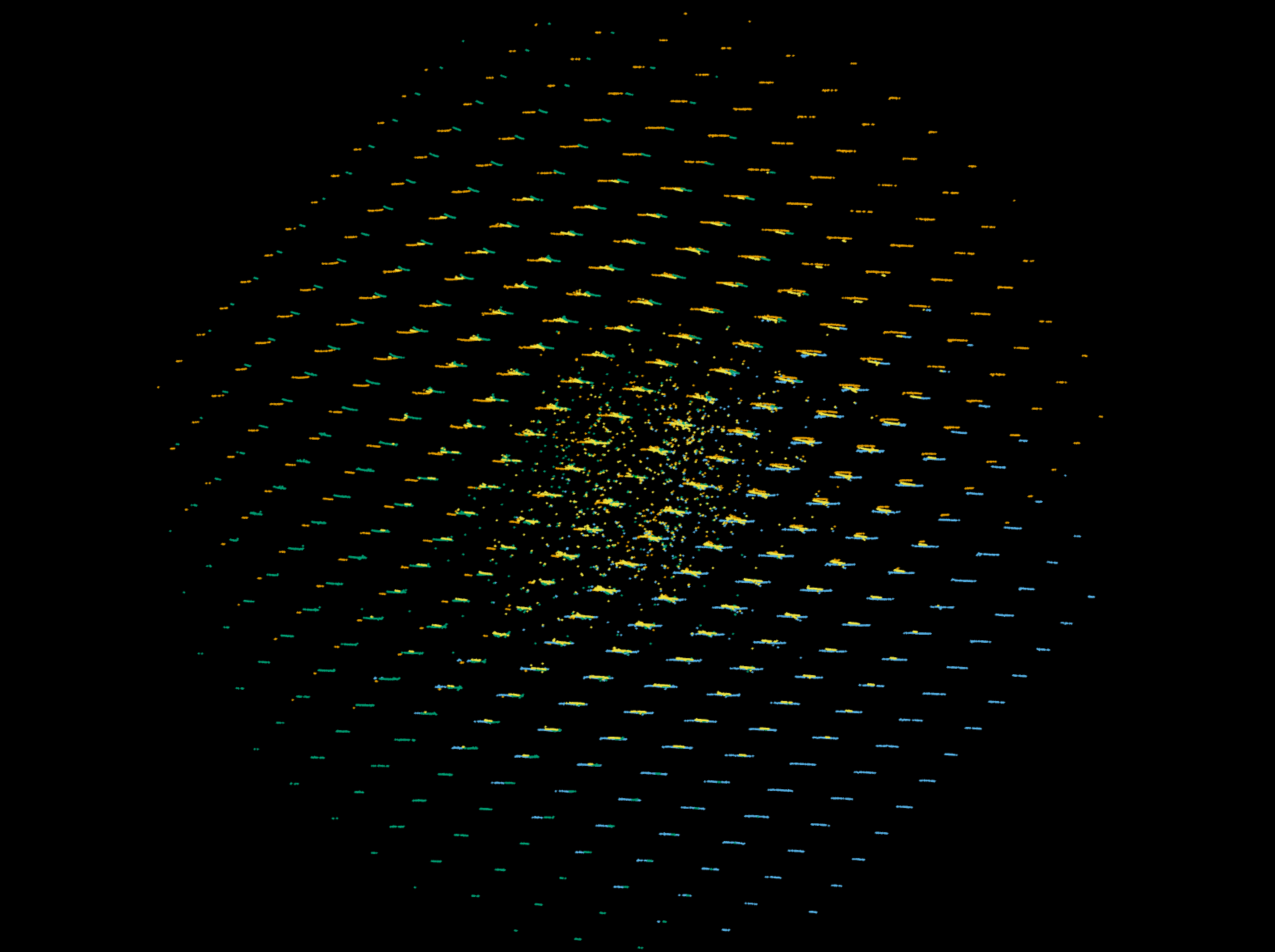
By default this will use all available cores, and may of course take a little while to work through four sequences. The spot finding is independent from sequence to sequence but the spots from all sequences may be viewed with
dials.reciprocal_lattice_viewer imported.expt strong.refl
Which will show how the four sequences overlap in reciprocal space, as:
Indexing
Indexing here will depend on the model for the experiment being reasonably accurate. Here the lattices overlap in the reciprocal lattice view above, the indexing should be straightforward and will guarantee that all lattices are consistently indexed as a single matrix is used.
Note
if the lattices do not align in reciprocal space for your data then processing sweeps independently is likely to be needed
dials.index imported.expt strong.refl
Without any additional input, the indexing will determine the most appropriate primitive (i.e. triclinic) lattice parameters and orientation which describe the observed reciprocal lattice positions.
Bravais lattice determination
Prior to refinement the choice of Bravais lattice may be made, though this is entirely optional and all processing may be performed with a triclinic lattice:
dials.refine_bravais_settings indexed.refl indexed.expt
Once this has run you can manually rerun indexing with:
dials.index imported.expt strong.refl space_group=P222
to assign the lattice, or manually reindex the data to match setting #5 (though in this case that is a no-op) - or as mentioned above proceed with the lattice unconstrained.
Note
if you are certain that the lattice symmetry is correct then the refinement should be more stable, and yield more reliable unit cell constants
Note
if you select an incorrect lattice then the subsequent processing may fail
Refinement
Prior to integration we want to refine the experimental geometry and the scan varying crystal orientation and unit cell: the calculations are performed first with a scan static model, then with scan varying (which allows for small variations in the sample orientation etc.) to account for impact of reindexing data prior to refinement.
dials.refine indexed.refl indexed.expt
At this stage the reciprocal lattice view will show a much improved level of agreement between the indexed reflections from the four sequences:
dials.reciprocal_lattice_viewer refined.expt refined.refl
If the Bravais lattice was assigned, in refinement the lattice constraints (here that all cell angles are 90 degrees) will be applied.
Integration
At this stage the reflections may be integrated. This is done by running
dials.integrate refined.refl refined.expt
which will integrate each sweep in sequence, again using all available cores. After integration you can look at the integration shoeboxes with the image viewer, as
dials.image_viewer integrated.refl integrated.expt
Symmetry Determination
So far the data were processed with a triclinic unit cell, which is usually OK but not ideal for correctly scaling the data. After integration it is usual to determine the symmetry for scaling using
dials.symmetry integrated.refl integrated.expt
This will look at the shape of the unit cell and determine the maximum possible symmetry based on the cell parameters, with some tolerance. Each of the possible symmetry operations will be individually tested and scored, and those operations identified as being present will be composed into the point group to be assigned to the data. An attempt is then made to estimate the space group from the presence or absence of axial reflections: this is rather less reliable than the point group determination but also less important for the scaling. After the point group has been determined the reflections will be reindexed automatically to match the correct setting, ensuring that the data are correctly prepared for scaling.
Note
dials.symmetry will only suggest one of the 65 Sohncke space groups relevant for chiral molecules. It will not detect mirrors or glide planes.
Scaling
In general there is very little which needs to be adjusted in the scaling, as the process is largely automatic. The default model to use for the scaling corrections is “physical” which defines smoothly varying scale factors for the overall intensity and sample decay, with a smoothly varying surface expressed with four or six orders of spherical harmonics for the absorption correction. For organic small molecule crystals the absorption is unlikely to be substantial, so the default is to set low absorption. If metals are present or the data are taken with a long wavelength it may be helpful to reduce the strength of the restraints on the absorption surface by setting the absorption level
dials.scale symmetrized.refl symmetrized.expt
dials.scale symmetrized.refl symmetrized.expt absorption_level=medium
At this stage it is reasonable to consider assigning a resolution limit to the data, though the tutorial data are strong to the edge - this is achieved by setting d_min=0.7 (as an example). Suggestions on a sensible resolution limit to use, based on the CC half value, are included in the program output.
At the end of the output is the summary of the merging statistics for all data passed as input
          -------------Summary of merging statistics--------------

                                             Overall    Low     High
High resolution limit                           0.58    1.58    0.58
Low resolution limit                           12.04   12.04    0.59
Completeness                                   96.9   100.0    49.4
Multiplicity                                    7.7    11.8     1.3
I/sigma                                        45.2    93.6     9.4
Rmerge(I)                                     0.030   0.024   0.076
Rmerge(I+/-)                                  0.029   0.023   0.067
Rmeas(I)                                      0.032   0.025   0.099
Rmeas(I+/-)                                   0.032   0.025   0.095
Rpim(I)                                       0.010   0.007   0.063
Rpim(I+/-)                                    0.012   0.008   0.067
CC half                                       1.000   1.000   0.985
Anomalous completeness                         90.9   100.0    10.1
Anomalous multiplicity                          4.6     8.5     1.1
Anomalous correlation                         0.168   0.137   0.000
Anomalous slope                               1.251
dF/F                                          0.023
dI/s(dI)                                      0.991
Total observations                            12198    1275      55
Total unique                                   1583     108      41
Here it is clear that the data are “good” across the detector though the outer shell is incomplete due to the experimental geometry. From a data processing perspective our work is done, however in terms of downstream analysis there is more we can do, e.g. determination of a good unit cell to use for the subsequent stages of processing (with ESDs) and transforming the data format for e.g. SHELX.
Unit cell refinement
After integration the unit cell for downstream analysis may be derived from refinement of the cell against observed two-theta angles from the reflections, across the four sequences:
dials.two_theta_refine scaled.refl scaled.expt p4p=scaled.p4p
Here the results will be output to a p4p file for XPREP, which includes the standard uncertainties on the unit cell. Since the data are already scaled however it is not necessary to do any further scaling e.g. with SADABS. If you do wish to scale the integrated data with SADABS, see below. The uncertainties in the unit cell parameters after integration are typically rather small:
Final refined crystal model:
Crystal:
    Unit cell: 5.42183(3), 8.13282(5), 12.02218(7), 90.0, 90.0, 90.0
    Space group: P 21 21 21
    U matrix:  {{ 0.6983,  0.2387, -0.6749},
                { 0.5789, -0.7429,  0.3362},
                {-0.4212, -0.6254, -0.6569}}
    B matrix:  {{ 0.1844,  0.0000,  0.0000},
                {-0.0000,  0.1230,  0.0000},
                {-0.0000, -0.0000,  0.0832}}
    A = UB:    {{ 0.1288,  0.0293, -0.0561},
                { 0.1068, -0.0913,  0.0280},
                {-0.0777, -0.0769, -0.0546}}
+-------------+-----------+----------------+
| Parameter   |     Value |   Estimated sd |
|-------------+-----------+----------------|
| a           |   5.42183 |        3e-05   |
| b           |   8.13282 |        5e-05   |
| c           |  12.0222  |        7e-05   |
| alpha       |  90       |        0       |
| beta        |  90       |        0       |
| gamma       |  90       |        0       |
| volume      | 530.115   |        0.00356 |
+-------------+-----------+----------------+
Saving refined experiments to refined_cell.expt
However these may be useful in later structure refinement.
Exporting
The output data are by default saved in the standard DIALS reflection format, which is not particularly useful. DIALS is able to convert this to SHELX format though. This can be done by
dials.export scaled.refl scaled.expt format=shelx shelx.ins=lcys.ins shelx.hklout=lcys.hkl composition=CHNOS
So that you can then run
shelxt lcys
to solve the structure etc.
Output for SADABS (alternate path)
After integration, the data should be split before exporting to a format suitable for input to XPREP or SADABS. Note that SADABS requires the batches and file names to be numbered from 1:
dials.split_experiments integrated.refl integrated.expt
dials.export format=sadabs reflections_0.refl experiments_0.expt sadabs.hklout=integrated_1.sad run=1
dials.export format=sadabs reflections_1.refl experiments_1.expt sadabs.hklout=integrated_2.sad run=2
dials.export format=sadabs reflections_2.refl experiments_2.expt sadabs.hklout=integrated_3.sad run=3
dials.export format=sadabs reflections_3.refl experiments_3.expt sadabs.hklout=integrated_4.sad run=4
If desired, p4p files for each combination of reflections_[0-3].refl, experiments_[0-3].expt could also be generated.