
Processing a Zn-SAD data set with DUI2 or the command line
Introduction
This tutorial takes you through processing a typical macromolecular crystallography data set with DIALS, from importing the images to exporting scaled intensities ready for structure solution. You can drive DIALS either from the DUI2 graphical user interface or by typing commands at a terminal. The crystallography is the same either way. Only the actions you take differ.
Wherever the two routes differ you will see a pair of tabs labelled DUI2 and Command line. Choose the tab for the route you are following. All the tabs on the page switch together, so you only need to choose once.
You are following the DUI2 route. Instructions in these tabs tell you which buttons to press in the DUI2 window.
You are following the command-line route. Instructions in these tabs tell you which DIALS commands to type at a terminal.
Data
To process the data locally with DIALS you will need a copy of the data set on
your computer. If you do not have it already you can download it from Zenodo:

Hint
If you are at a DIALS workshop please ask your tutor where to find the data set, which might already be downloaded for you.
We will use the Zinc K edge data set, which consists of 800 images named
ADH4_M7S9_6_0001.cbf to ADH4_M7S9_6_0800.cbf (ADH4 is an old
name for the gene encoding the protein).
Summary
We will work on a data set recorded from crystals of the enzyme tetrahydroalstonine synthase (THAS1), with thanks to Prof. Dave Lawson for providing the data set. The images were collected at Diamond Light Source on a PILATUS 6M pixel array detector at an X-ray wavelength of 1.282 Å, at the Zinc K edge. There is sufficient anomalous signal to solve the structure by experimental phasing (SAD). There are some more details about the data set in the Zenodo deposition.
First we will set up a xia2 processing job, running remotely on the CCP4 Cloud at Harwell. This keeps your local computer free to process the data at the same time with DIALS, using either DUI2 or the command line.
Once you have finished the interactive processing, you can compare your results with the xia2 job. Are there any differences? Which job has better statistics?
Processing with xia2 on CCP4 Cloud
If you have the CCP4 icons available, double click on the icon named “CCP4Cloud Remote”. Alternatively, in a terminal with the CCP4 environment sourced, run the script ccp4cloud-remote. This opens a web browser where you can log in to the CCP4 Cloud at Harwell. Here we assume you already have an account and know how to create a new project.
To process the images on CCP4 Cloud the images must be available on Cloud. You could upload the data set from your computer, but that would take a long time, and the data set is already publicly available on Zenodo. Instead, we can tell Cloud to fetch the data directly from Zenodo. If the data set is already in your Cloud storage, skip ahead to the xia2 job.
Start a new task in your Cloud project. Open the “Data Import” folder in the
“All tasks” list and select “Fetch diffraction images from WWW repositories”
from the “Upload to Cloud Storage” section. Enter
https://doi.org/10.5281/zenodo.21258293 as the DOI code and start the
job.
Now add a new “Automatic Image Processing with Xia-2” task. Under “Input Data”,
make sure the task will “Look for X-ray images in cloud storage”. Browse for the
image directory, navigating to
My Cloud Storage/zenodo/21258293/images/Zinc_K_edge_data. Then click on
the directory images_1-800 and “Select” it (do not “Open” it). Set a
sensible project and crystal name, and don’t forget to add “Zn” as the heavy
atom type! There’s no need to set any advanced options, just press “Run”. Make
sure the job starts, but after that you can leave it to process while you work
on the images locally with DIALS.
Warning
Image data uploaded to Cloud is large and will eventually be deleted to save space. So don’t consider CCP4 Cloud as a backup solution for your diffraction data!
Setting up DIALS processing
We will process the images with DIALS through DUI2. You can start DUI2 in either of two ways:
If DUI2 is installed as an app on your computer (for example, on Windows), launch it from your desktop’s application menu. On Windows, click the Start button and type “DUI2”, then click the DUI2 entry. Don’t worry if nothing seems to happen! DUI2 starts slowly. Eventually it will ask you to select a directory to work in.
Alternatively, open a terminal with the CCP4 environment sourced. Opening a terminal differs by operating system. Please ask for help if you are unsure how to do this. Change to a directory where you want to do the processing (we recommend a different directory from the one holding the images), then start dui2. For example, using BASH on Linux or Mac:
cd ~
mkdir THAS1-dials
cd THAS1-dials
dui2
or at the Windows command prompt:
cd %USERPROFILE%
mkdir THAS1-dials
cd THAS1-dials
dui2
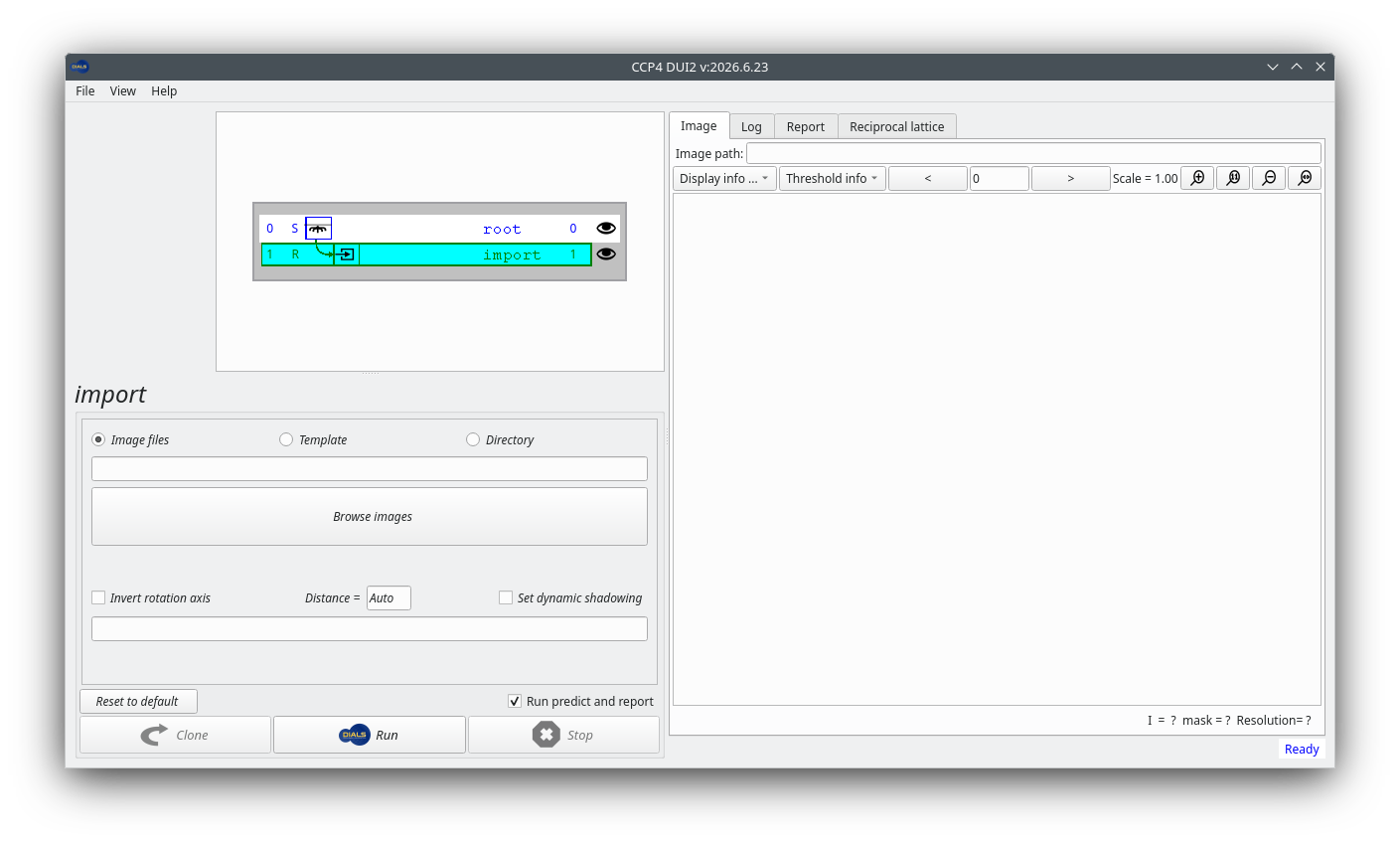
Once the program starts you should see something like this:
We will process the images by running DIALS commands at a terminal. In a terminal with the CCP4 (or DIALS) environment sourced, first change to a directory where you want to do the processing (we recommend a different directory from the one holding the images):
cd ~
mkdir THAS1-dials
cd THAS1-dials
Importing the images
The first task in data processing with DIALS is to import the images, using the program dials.import.
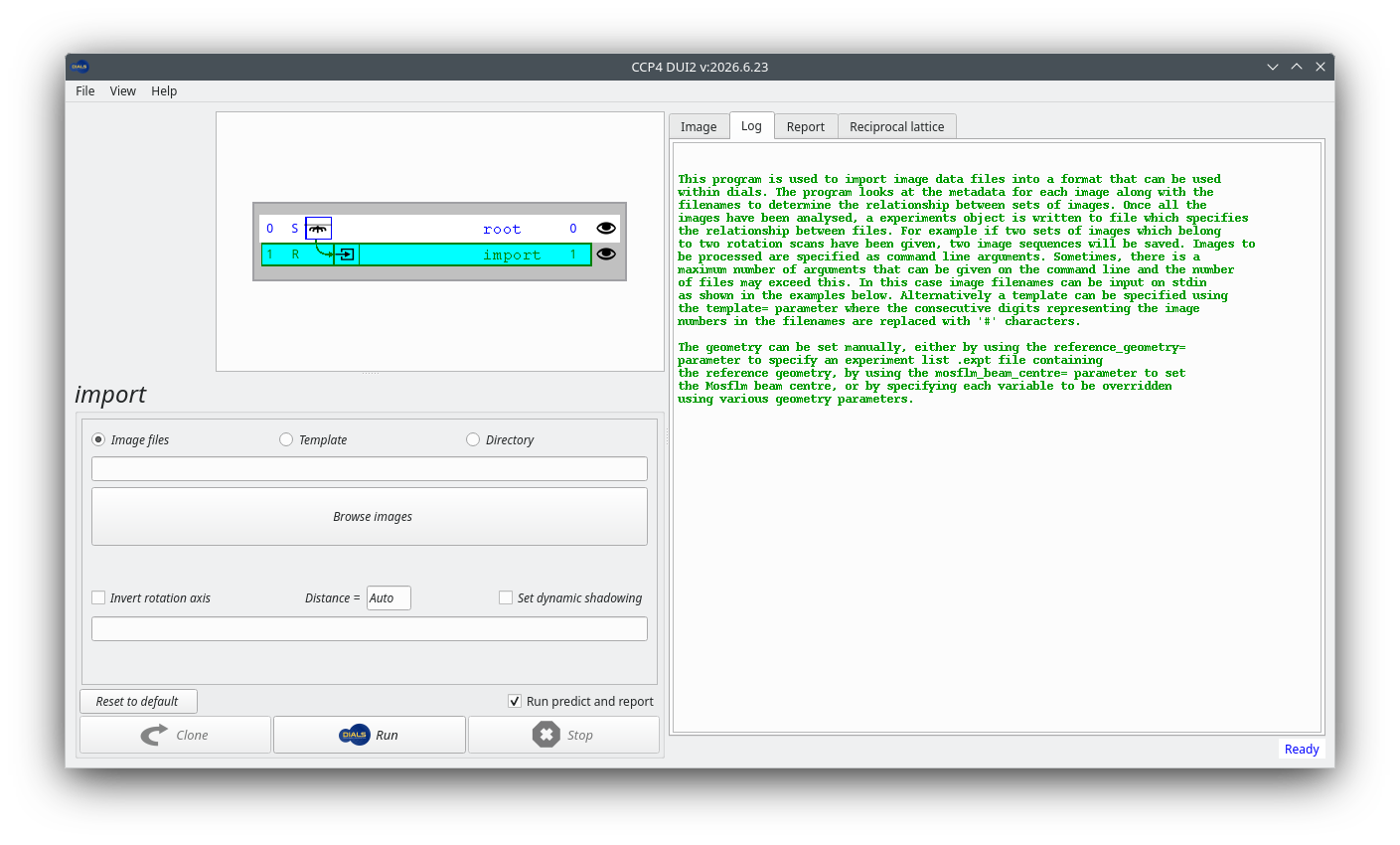
The DUI2 history tree already highlights an incomplete import
node. To see some help for a node that hasn’t yet been run, click on
the “Log” tab on the right. Note that this help message mainly
describes running dials.import from the command line, so
some of it might not apply to DUI2.
To import the data set, click on the “Open images” button and navigate
to the directory where the images are located. Click on just one of
the CBF images, say ADH4_M7S9_6_0001.cbf, and then click
“Open”. DUI2 automatically converts that to a template that matches
all the images in the data set.
Note
For EIGER data there is not one file per image, but usually a few
files with the extension .h5. In this case, just select the
file with the name that ends _master.h5, or, better, the
file with the extension .nxs if there is one.
DUI2 has not actually done the import yet. To do that, click on the “Run” button with the DIALS logo, at the bottom of the window. Once the job has finished, the “Log” tab shows output like this:
Like other dials.something commands, running the program without
options prints a help message with some usage examples:
dials.import
You may have to scroll up to read the full output. If you add the
option -h to this command you will see not only the help message,
but also the structured definitions of the command line parameters
that you can pass to the program.
Hint
What happens if you pass multiple h and v characters? Try
this out later with other DIALS programs too.
Now import the images with the following command, after adjusting the path to the files on your computer:
dials.import /path/to/images/ADH4_M7S9_6_*.cbf
Note the use of the wildcard * character in the
dials.import command. This is not DIALS syntax: the shell
expands it to match every image file in that directory, from
ADH4_M7S9_6_0001.cbf to ADH4_M7S9_6_0800.cbf.
dials.import reads the header of each of these files,
checks the diffraction geometry, and determines the relationship
between the files.
Note
For EIGER data there is not one file per image, but usually a few
files with the extension .h5. In this case, just pass the
file with the name that ends _master.h5, or, better, the
file with the extension .nxs if there is one.
If all goes well you will see output that looks something like this:
--------------------------------------------------------------------------------
  format: <class 'dxtbx.format.FormatCBFMiniPilatusDLS6MSN100.FormatCBFMiniPilatusDLS6MSN100'>
  template: /data/THAS1/images_1-800/ADH4_M7S9_6_####.cbf:1:800
  num images: 800
  sequences:
    still:    0
    sweep:    1
  num stills: 0
--------------------------------------------------------------------------------
Writing experiments to imported.expt
This tells you that DIALS interprets the 800 images as a single rotation sweep.
It writes the diffraction geometry and associated metadata to a new file,
imported.expt.
You can see a summary of the experimental models, including the detector and beam geometry, in the HTML report available from the “Report” tab, under the “Experiments” heading.
To get human-readable information from that file, try:
dials.show imported.expt
Viewing the images
Whichever route you take, you should look at the images!
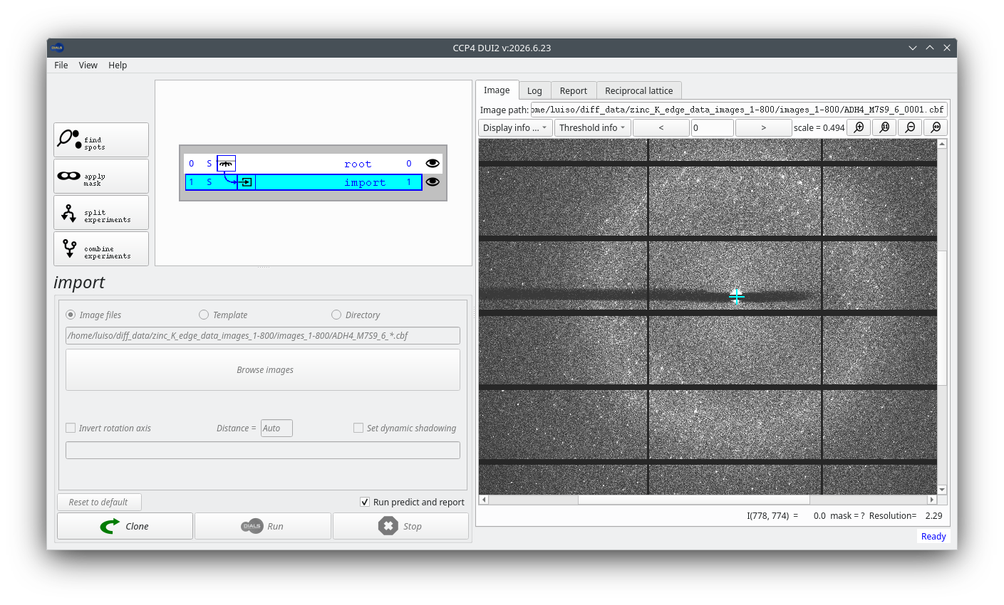
Click on the “Image” tab to view the diffraction images in DUI2’s viewer. If you have a mouse wheel you can use it to zoom, or use the magnifying glass buttons at the upper right of the window. Click and drag to scroll the image. More options to change the contrast and colour scheme are in the “Display info” pull-down menu.
DIALS contains a feature-rich image viewer for this purpose:
dials.image_viewer imported.expt
Take a moment to explore the controls in the image viewer. Can you drag the image around and zoom using the mouse? Can you see the intensity and resolution information for a single pixel? What is your preferred colour scheme and brightness? Can you scroll through and see how the diffraction images change as data collection proceeds? Don’t be afraid to play with the controls. Nothing you do here will affect processing of the data set.
Hint
Look at images at various points in the data set: at the beginning, in the middle, and at the end. Does the crystal diffract well throughout? Are there any other features present alongside the diffraction spots?
Masking the backstop shadow (optional)
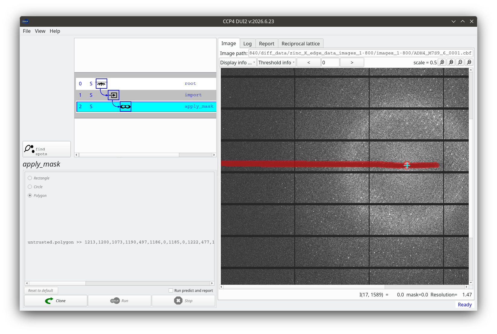
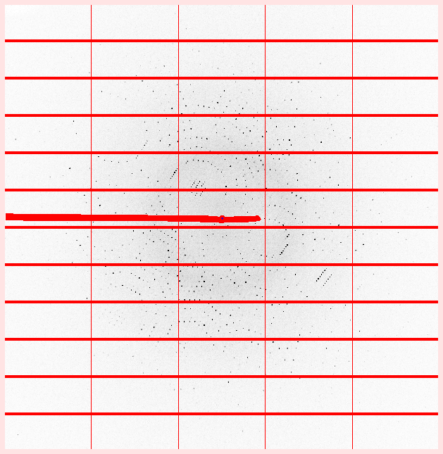
There is a horizontal backstop shadow across the images. We could mask it out if we wanted, but the rotation axis is aligned with the backstop shadow. (You can see the rotation axis in dials.image_viewer, but not in the DUI2 viewer.) Spots close to the rotation axis are less reliable and will not be integrated anyway. Can you work out why?
Nevertheless, if you want to try it, you can mask out the shadow. Click the “apply mask” button and choose one of the options (we recommend “Polygon”), then click in the image to define a mask. Be aware that the mask is not actually applied until you click the DIALS “Run” button! After that the masked region is displayed in translucent red, like this:
Nevertheless, if you want to try it, you can mask out the shadow using
the image viewer. First increase the brightness to make the shadow
more visible. A value of 100 should do fine. Then zoom into the image
to make it easier to click around the edge of the shadow. A zoom level
of 100% is likely to make the shadow fill the width of your screen.
Now, in the “Actions” menu at the top of the main image viewer window,
select “Show mask tool”, and then choose one of the modes (we
recommend “Polygon”). Now click around the edge of the shadow. When you
have finished, select a different mode (say “Circle”) to ensure that
the polygon has been completed. Finally click the “Save” button to
save the mask definition to the file mask.phil, and close the
image viewer.
To actually set the defined mask in the experiments file, run these commands:
dials.generate_mask imported.expt mask.phil
dials.apply_mask imported.expt mask=pixels.mask
If you now open the new file with the image viewer
(dials.image_viewer masked.expt) and click “Show mask” in the
main controls, you will see that the backstop shadow mask has been
combined with the default mask for the module gaps.
Note
In the commands that follow, use masked.expt if you masked
the backstop, or imported.expt if you did not.
Finding spots
Click the “find spots” button to move to the next step. You can adjust various parameters that control the spot-finding algorithm. For PILATUS data sets like this one the default parameters are usually sensible, so just click the “Run” button to start the job.
With the image viewer open, select the “Threshold pixels” checkbox. This shows you which pixels the spot-finding algorithm considers to be “strong”.
Hint
Do the strong pixels match the position of the diffraction spots? What happens if you change parameters of the threshold algorithm (like kernel size and gain)? What happens if you select different threshold algorithms?
The default parameters seem pretty good for this data set, so exit the image viewer and run a default spot-finding job:
dials.find_spots masked.expt
If you did not mask the backstop, use imported.expt in place
of masked.expt here and in the later commands.
DIALS finds spots throughout the entire rotation scan, whereas some other programs default to finding spots on just enough images to perform indexing. This means spot-finding takes longer with DIALS, but the information determined from the entire scan can be reused multiple times. In fact, DIALS will not need to read the image data again until integration. At the end of the spot-finding procedure the log shows an ASCII-art histogram of the number of spots found on each image. In this case it is pretty boring because the crystal diffracts consistently well throughout the scan:
Histogram of per-image spot count for imageset 0:
307302 spots found on 800 images (max 5525 / bin)
*                                * **** ** * * **  ** *    *
************************************************************
************************************************************
************************************************************
************************************************************
************************************************************
************************************************************
************************************************************
************************************************************
************************************************************
1                         image                          800

--------------------------------------------------------------------------------
Saved 307302 reflections to strong.refl
Similar information is available graphically from the “Report” tab. Click on the button to open the report in a web browser, then click on “Analysis of strong reflections” to see the per-image counts. You can also see details of the experiment geometry by clicking on the “Experiments” heading to expand the box.
You can see similar information graphically by generating an HTML report:
dials.report masked.expt strong.refl
Open dials.report.html in a web browser and click on “Analysis
of strong reflections” to see the per-image counts.
Viewing the reciprocal lattice
The dials.reciprocal_lattice_viewer displays the positions of the strong spots mapped into reciprocal space.
DUI2 does not contain its own reciprocal lattice viewer, but it can launch dials.reciprocal_lattice_viewer for you, from a button in the “Reciprocal lattice” tab. Press that button.
Pass both the experimental geometry file (masked.expt or
imported.expt) and the spot file strong.refl to
dials.reciprocal_lattice_viewer:
dials.reciprocal_lattice_viewer masked.expt strong.refl
Hint
Use tab completion, if your shell supports it, to avoid typing out long commands or filenames like dials.reciprocal_lattice_viewer. Even without tab completion, in this case you can use the alias dials.rlv instead.
Take some time to explore the controls in the dials.reciprocal_lattice_viewer.
Hint
What does middle-button drag do? Try setting “Max Z” to something small, like 5. What does this show you? Align the view down the rotation axis and then click to increase the Max Z value (use Alt-click to jump in blocks of 100). Can you see how data collection sweeps out a volume of reciprocal space? Can you align the view in a direction that clearly shows the crystal lattice?
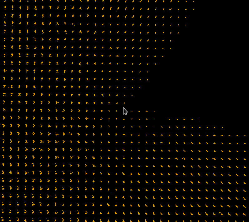
Before indexing, the main purpose of the dials.reciprocal_lattice_viewer is to look for pathologies that might cause indexing to fail, such as poor diffraction geometry, noisy spots, split spots, ice rings, and so on. In this case the reciprocal lattice looks very clean. Here is a view with a nicely aligned lattice, suggesting that indexing should not be a problem:
Indexing
By default, dials.index will find a \(P\,1\) cell, using the 3D FFT algorithm.
Click the “index” button to set up a dials.index job. The
default settings are fine for our purposes, but feel free to
experiment with the others. If a job goes wrong you can always click
back to the find_spots node on the history tree and start a new
“index” job from that point. Click “Run” to start the job.
It is worth taking a moment to read the output in the “Log” tab once the job completes.
Run a default dials.index job:
dials.index masked.expt strong.refl
It is worth taking a moment to read the log output.
The program runs through a few stages:
Setting up for indexing (calculating
max_cell, setting resolution limits, mapping spots to reciprocal space and forming the FFT grid)Performing the FFT, searching for real space basis vectors and forming candidate solutions (in this case 50)
Ranking the solutions and choosing the single best
Performing geometry refinement in macrocycles with increasing resolution. At each stage this:
Identifies outliers
Parameterises the diffraction geometry
Refines this geometry against the observations
Increases resolution for the next macrocycle
Once the resolution limit includes all reflections, writing the final refined model and reflections to the files
indexed.exptandindexed.refl
Parameters given to dials.index control the behaviour of all of these stages, but in most cases the defaults are fine.
Now we have a crystal model it is worth looking at the reciprocal lattice again.
Launch the dials.reciprocal_lattice_viewer from the “Reciprocal lattice” tab.
dials.reciprocal_lattice_viewer indexed.expt indexed.refl
The spots are now coloured according to whether they are indexed or not, although in this case almost all spots are indexed.
Hint
Try the “Show reciprocal cell” option. Zoom in and see if you can align the view with one of the reciprocal basis vectors, \(a^\star\), \(b^\star\) or \(c^\star\). Try the toggles between “indexed” and “unindexed”, “inliers” and “outliers”.
Back in the DUI2 main window, switch to the “Image” tab. Now that we
have a crystal model, you can switch between displaying shoeboxes for
the observed spots and little “+” symbols for the predicted spots
(see the “Display info” pull-down). At a high enough zoom level the
viewer also displays the Miller indices of the reflections.
You can also view the indexed spots and the predictions on the images,
by running dials.image_viewer indexed.expt indexed.refl. Try
the “Show predictions” and “Show miller indices” options.
Determining the Bravais lattice
The initial solution from dials.index is triclinic, but the α, β and γ angles are very close to 90°. To identify compatible Bravais lattices we run dials.refine_bravais_settings. This enforces the Bravais symmetry of compatible lattices (within some tolerance) and runs refinement.
Click on the “refine bravais settings” button and press “Run”. The results are printed as a table at the end of the log shown in the “Log” tab:
dials.refine_bravais_settings indexed.expt indexed.refl
Hint
Like dials.reciprocal_lattice_viewer, dials.refine_bravais_settings has a short alias: dials.rbs
The results are printed as a table:
Chiral space groups corresponding to each Bravais lattice:
aP: P1
mP: P2 P21
oP: P222 P2221 P21212 P212121
+------------+--------------+--------+--------------+----------+-----------+-------------------------------------------+----------+----------+
|   Solution |   Metric fit |   rmsd | min/max cc   |   #spots | lattice   | unit_cell                                 |   volume | cb_op    |
|------------+--------------+--------+--------------+----------+-----------+-------------------------------------------+----------+----------|
|   *      5 |       0.0338 |  0.078 | 0.904/0.947  |    12000 | oP        | 57.10 102.19 112.16  90.00  90.00  90.00  |   654423 | a,b,c    |
|   *      4 |       0.0338 |  0.078 | 0.947/0.947  |    12000 | mP        | 102.18  57.10 112.16  90.00  89.99  90.00 |   654379 | -b,-a,-c |
|   *      3 |       0.0336 |  0.078 | 0.947/0.947  |    12000 | mP        | 57.10 112.16 102.19  90.00  90.00  90.00  |   654411 | -a,-c,-b |
|   *      2 |       0.0083 |  0.071 | 0.904/0.904  |    12000 | mP        | 57.11 102.19 112.18  90.00  89.97  90.00  |   654619 | a,b,c    |
|   *      1 |       0      |  0.071 | -/-          |    12000 | aP        | 57.11 102.19 112.18  89.99  89.97  90.01  |   654702 | a,b,c    |
+------------+--------------+--------+--------------+----------+-----------+-------------------------------------------+----------+----------+
The choice of solution is down to the user, but solutions deemed acceptable are
marked as such. In general, we look for the highest symmetry solution with
reasonable values for the Metric fit, rmsd and min/max cc columns.
Here we will take solution 5, the primitive orthorhombic (oP) one.
To get appropriately reindexed reflections we run the program
dials.reindex, passing the change of basis operator printed in the
last column of the table. For solution 5 that operator is just a,b,c, which
is the identity: the reflections come out with the same indices as they go in.
So reindexing is not strictly necessary here, but we show the step anyway
because it usually is.
In DUI2 it is easier to see the table in the next step, reindexing. Click on the “reindex” button. The input pane now shows the same information as the text table, with a recommended solution highlighted.
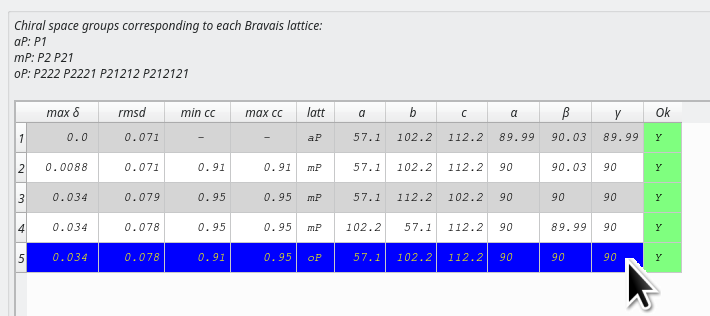
Acceptable solutions are marked with a “Y” in the “Ok” column. Make sure the row for solution 5 is highlighted and then press “Run”. DUI2 takes care of both selecting the Bravais lattice and reindexing the reflections.
dials.refine_bravais_settings marks acceptable solutions
with an asterisk: *. It writes out the experimental geometry for
every solution (files bravais_setting_1.expt to
bravais_setting_5.expt), but not the associated reflections.
The reflection files are larger, and there is no point wasting disk
space on solutions that will not be taken further. To reindex the
reflections for solution 5:
dials.reindex indexed.refl change_of_basis_op=a,b,c
This writes the file reindexed.refl.
The space group is now \(P\,2\,2\,2\). You can check this in the crystal model section of the HTML report. No attempt has been made yet to locate screw axes. That’s not a problem: we do not need to know the exact space group before integration, just a subgroup. There will be another attempt at symmetry determination later.
Refining the solution
We did some refinement during indexing, and again during Bravais lattice determination. Nevertheless, it is still worth running an additional step of refinement using the program dials.refine. This uses a more sophisticated outlier rejection algorithm than before. It also refines a “scan-varying” model of the crystal, in which the orientation and unit cell may change as a function of position in the rotation scan.
Click on the “refine” button and click “Run”.
Using the chosen Bravais lattice and our (unnecessarily) reindexed reflections, type:
dials.refine bravais_setting_5.expt reindexed.refl
From the log you should see that initially 13 parameters are refined during the “scan-static” macrocycle. This is followed by a “scan-varying” macrocycle using 37 parameters. Here the crystal parameters are made local to regions of the scan and the model is constructed by smoothing between these points. This more sophisticated model fits the predictions to the data better, and you should see lower RMSDs as a result. For example:
RMSDs by experiment:
+-------+--------+----------+----------+------------+
|   Exp |   Nref |   RMSD_X |   RMSD_Y |     RMSD_Z |
|    id |        |     (px) |     (px) |   (images) |
|-------+--------+----------+----------+------------|
|     0 | 254417 |   0.2914 |  0.28382 |     0.1768 |
+-------+--------+----------+----------+------------+
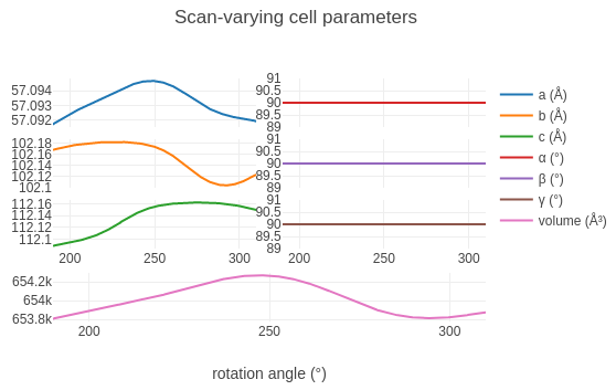
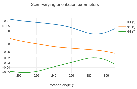
It is useful to look at the way the crystal parameters change during the scan, to make sure there are no unrealistic-looking changes.
Click on the “Report” tab, open the report, and expand the “Analysis of scan-varying crystal model” section.
Generate an HTML report for the refined model:
dials.report refined.expt refined.refl
This produces dials.report.html, containing plots and a lot
more information about the current stage of the data processing. Open
it in a web browser and expand the “Analysis of scan-varying crystal
model” section.
Alternatively, dials.plot_scan_varying_model refined.expt
writes similar plots as .png files.
You should see plots like these:
Hint
Check that the changes in unit cell parameters and orientation angles look small across the whole scan.
Integration
We now have a model for how the data set evolves over the whole scan. We are ready to use it to integrate every spot, including the weak ones that were not found during spot-finding. Integration is the most resource-intensive part of processing and takes the longest. After starting this job, maybe now is a good time to check on the progress of the xia2 job running on CCP4 Cloud.
Click on the “integrate” button and then “Run” to start a job with default parameters. You can switch to the “Log” tab to follow what stage the program is at.
dials.integrate refined.expt refined.refl
After predicting reflections, dials.integrate builds a model to determine how big the measurement boxes should be. This is printed to the log at the lines:
Calculating E.S.D Beam Divergence.
Calculating E.S.D Reflecting Range (mosaicity).
 sigma b: 0.041727 degrees
 sigma m: 0.062834 degrees
The sigma m value is the standard deviation of the reflecting range of
reflections, which is sometimes (and inaccurately) called “mosaicity”. It is
good to check that this value is not too high. Here it is well below 0.1°, so
the sample seems very well behaved.
After this step, dials.integrate splits the processing over as many processors as you have available. It first models reflection profiles, and then performs the actual integration, using both summation integration and profile fitting methods. There are some summary tables at the end of the log that are worth a glance, but we won’t have a good idea of the quality of the data set until we do scaling.
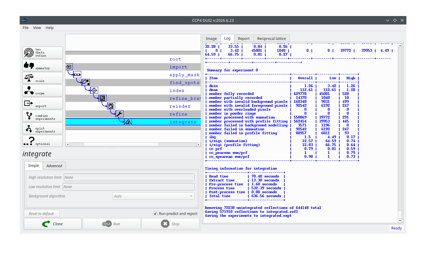
Once integration has finished, the report available from the “Report” tab contains new information, in the “Analysis of reflection intensities” and “Analysis of reference profiles” sections under “DIALS analysis plots”.
Running dials.report integrated.expt integrated.refl produces
a report with new information, in the “Analysis of reflection
intensities” and “Analysis of reference profiles” sections under
“DIALS analysis plots”.
Determining the crystal symmetry
Now we have integrated reflections we have much more useful data for symmetry checks. The program dials.symmetry first checks the Laue group (we hope this confirms our earlier choice of Bravais lattice). Then it looks for potential screw axes by looking for apparent systematic absences.
Click the “symmetry” button and “Run” for default parameters.
dials.symmetry integrated.expt integrated.refl
The systematic absence information is written to a table in the log:
+--------------+---------+---------------+--------------+---------------+--------------+-------------------+------------------+
| Screw axis   |   Score |   No. present |   No. absent |   <I> present |   <I> absent |   <I/sig> present |   <I/sig> absent |
|--------------+---------+---------------+--------------+---------------+--------------+-------------------+------------------|
| 21a          |       0 |            10 |           10 |       1253.16 |      340.318 |            35.204 |           17.228 |
| 21b          |       1 |            30 |           30 |       1575.34 |        1.901 |            45.998 |            0.318 |
| 21c          |       1 |            38 |           39 |       1167.44 |        3.281 |            74.032 |            1.487 |
+--------------+---------+---------------+--------------+---------------+--------------+-------------------+------------------+
Here we see clear screw axes along b and c. Reflections that are expected to
be present have high average intensity and \(I/\sigma\), while the absences
have low values. For the potential screw axis along a, the expected present
reflections do have higher intensity and \(I/\sigma\) than the absences, but
the intensity in the putative absences is actually rather high. This indicates
that a screw axis along a is not supported by the data. As a result,
dials.symmetry writes the files symmetrized.expt and
symmetrized.refl, using the space group \(P\,2\,2_1\,2_1\).
Note
\(P\,2\,2_1\,2_1\) is a non-standard setting of the space group \(P\,2_1\,2_1\,2\), which is how the deposited structure of THAS1 (PDB entry 5FI3) is described. The two differ only in how the axes are labelled, so the reflections must be reindexed (with the cell axes permuted) to go from one setting to the other. Downstream structure solution software can do this reindexing, so we don’t need to worry about it here.
Scaling
The scaling program, dials.scale, uses algorithms similar to Aimless to fit a physically interpretable scaling model to the data set. The model has three components:
an overall rotation angle-dependent scale factor (accounting for beam intensity changes, variation in illuminated volume and similar effects)
a relative B-factor decay term (accounting roughly for the loss of high resolution reflections caused by radiation damage)
an absorption surface (accounting for absorption along the differing path lengths of scattered rays through the crystal volume)
The parameters of these components are adjusted to minimise the differences between reflections and their symmetry mates (which ought to have the same intensity). While performing this fit, dials.scale also optimises an error model so that the error associated with the merged intensity of each reflection group is appropriate. We run the program with default options.
Click on the “scale” button and then “Run”.
dials.scale symmetrized.expt symmetrized.refl
At the end of the log a standard table of merging statistics is printed. Parts of it may be familiar to you from “Table 1” of crystallographic structure papers:
            -------------Summary of merging statistics--------------

                                             Overall    Low     High
High resolution limit                           1.26    3.42    1.26
Low resolution limit                          112.16  112.61    1.28
Completeness                                   82.6    97.7     5.8
Multiplicity                                    3.8     4.3     1.0
I/sigma                                        15.0    44.2     0.8
Rmerge(I)                                     0.066   0.050   0.625
Rmerge(I+/-)                                  0.054   0.043   1.675
Rmeas(I)                                      0.075   0.056   0.884
Rmeas(I+/-)                                   0.068   0.053   2.369
Rpim(I)                                       0.034   0.026   0.625
Rpim(I+/-)                                    0.041   0.031   1.675
CC half                                       0.997   0.995   0.370
Anomalous completeness                         69.8    91.7     0.1
Anomalous multiplicity                          2.1     2.4     1.0
Anomalous correlation                         0.131   0.074   0.000
Anomalous slope                               1.124
dF/F                                          0.071
dI/s(dI)                                      1.255
Total observations                           561027   39438     526
Total unique                                 145885    9107     507
Hint
Do the summary statistics look okay? Is there any sign of an anomalous signal?
The summary table is worth a quick glance, but graphical representations of the merging statistics are usually more informative.
The report from the “Report” tab now contains plots of values against resolution and against image number.
Open the file dials.scale.html in a web browser to see plots
of values against resolution and against image number.
Hint
Look at the plots in the report. What is the main factor determining the usable resolution limit in this case? How does the anomalous signal look?
Exporting
Although dials.scale reports the merging statistics, the data set has not actually been merged (merging keeps only a single record for each unique Miller index). We could export a merged MTZ for structure solution using dials.merge. In our case, however, we prefer to export the scaled, unmerged data with dials.export and then merge inside CCP4 Cloud, so that the merging statistics are also recorded there.
If you wanted a merged MTZ, you would click on the “merge” button and
export merged.mtz. Instead, to export the unmerged data, click
on the “export” button and click “Run”. Once that is finished, click
on the “Download/save file” button to save the file to the directory
where you started the processing.
You can also upload the exported MTZ directly to CCP4 Cloud. To do that you need some information from Cloud. Go to your Cloud account and note the current project ID. Then click on the menu icon in the top left corner, and select “My Account”.
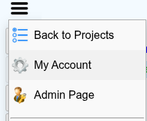
On the page that opens, note your login name and copy the “CloudRun Id” value.
Now, back in DUI2, press the “Upload to CCP4-cloud” button. Fill in the required fields in the pop-up window. If you are uploading to an existing project specified by ID, the value you give for “Project name” does not matter, but it cannot be left blank.
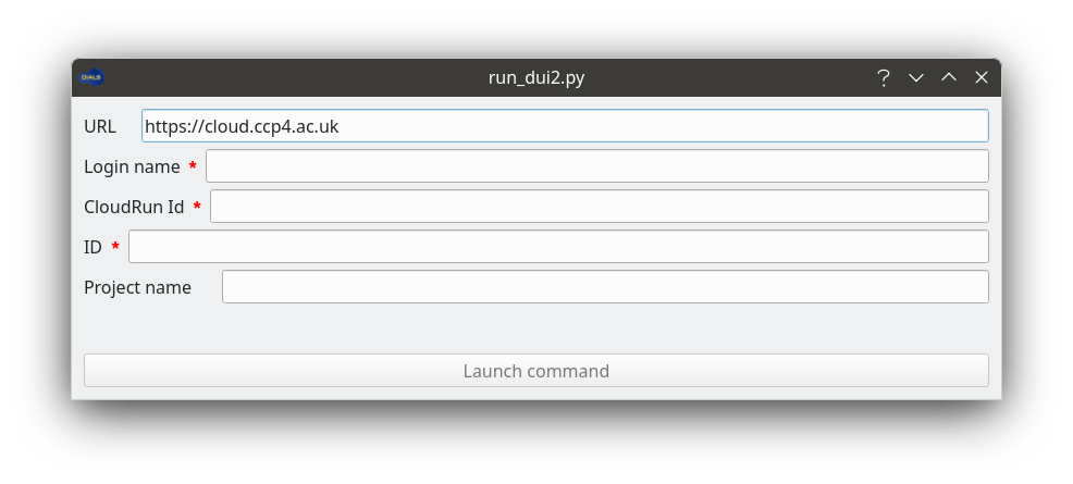
When the upload finishes, DUI2 creates a new cloudrun node, which
runs the file import task on the MTZ in your Cloud project.
Note
The “Upload to CCP4-cloud” button relies on the cloudrun
program from a local CCP4 installation. If you installed DUI2
standalone, the button will fail or be unavailable. In that case
upload the MTZ file manually through the CCP4 Cloud website, as
described below.
If you wanted a merged MTZ, you would run:
dials.merge scaled.expt scaled.refl
Instead, to export the unmerged data:
dials.export scaled.expt scaled.refl
This produces the file scaled.mtz, which we will upload to
CCP4 Cloud through the CCP4 Cloud website, as described below.
Uploading an MTZ file to CCP4 Cloud manually
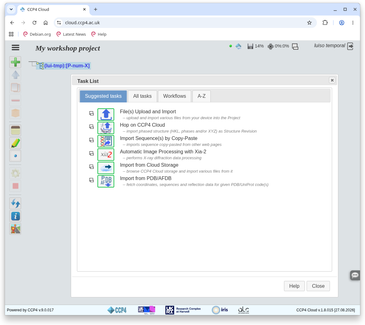
In CCP4 Cloud, open your project’s task list and click “File(s) Upload and Import” to create a new upload task.
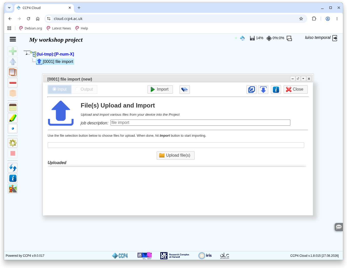
The task opens a “File import (new)” dialog. Click “Upload file(s)”.
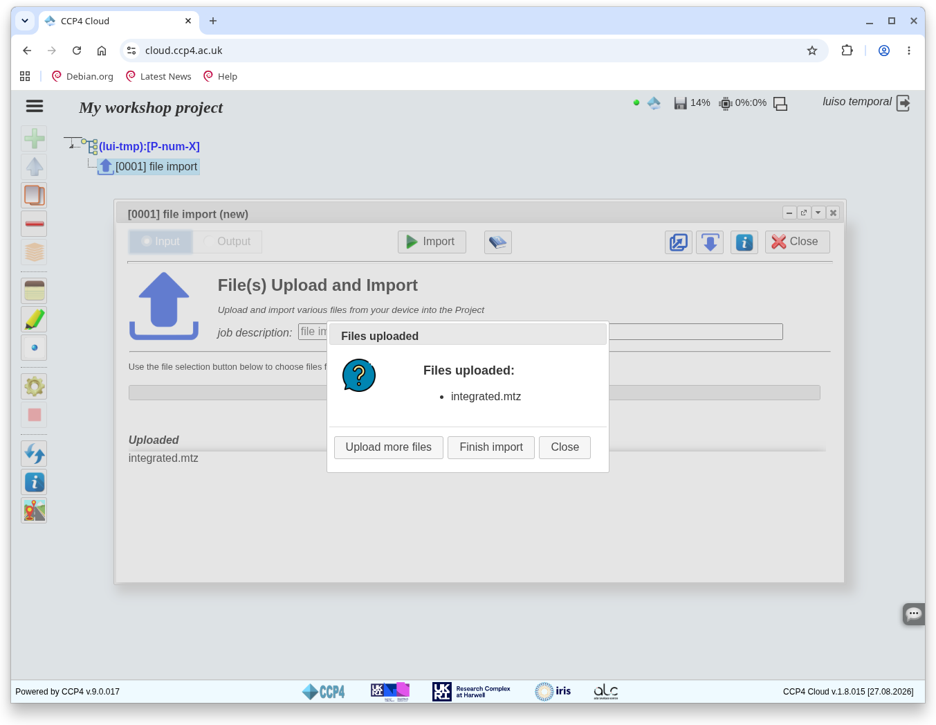
Choose your exported MTZ file in your computer’s file browser. Once it has uploaded, a new dialog appears on top of the previous one. Click “Close”.
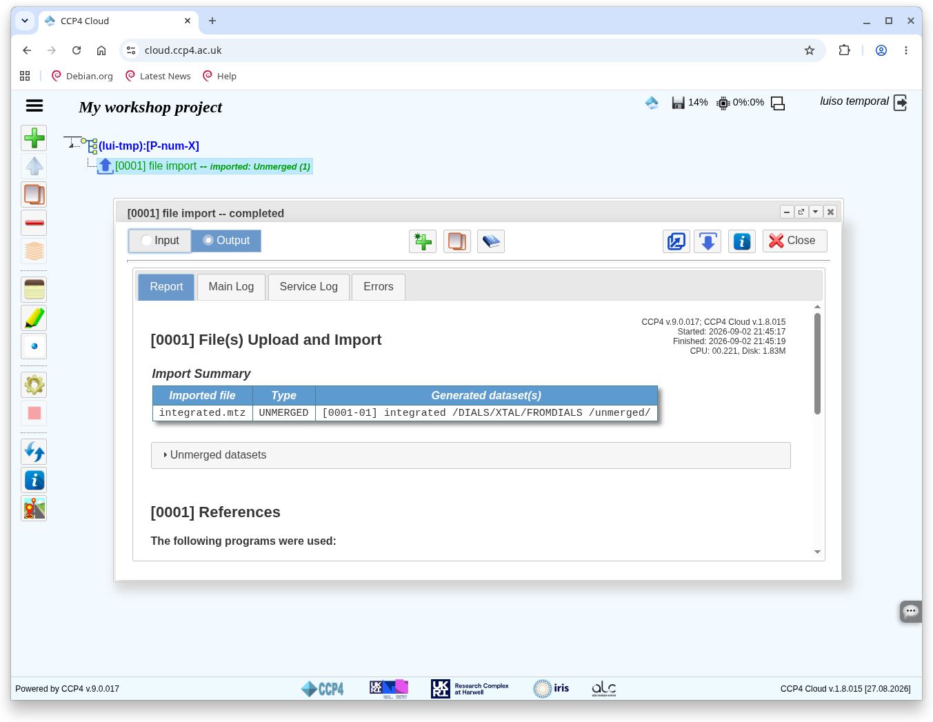
The “File import” dialog now reads “completed” and lists the uploaded file in a table. Your MTZ is now in the CCP4 Cloud project.
Comparing results with xia2
Hopefully by now the xia2 job you started on CCP4 Cloud has finished. Following that job, run a “Merging and Scaling with Aimless” job, and under “Basic Options” select “no scaling only merge”. Leave everything else as default and run.
Now follow your imported DIALS MTZ (from either the manual upload or the
cloudrun upload) with another “no scaling only merge” Aimless job.
Once both jobs have finished, open both results windows to compare results side by side. Navigate to the “Scaling and merging” section in each case to compare merging statistics from Aimless.
Which job looks better, yours or xia2’s? Or are they about the same?