Important

This tutorial requires DIALS >= 3.24.0. It will not work for earlier versions of DIALS.

Intensity-Based Clustering

Introduction

A key component of multi-crystal data analysis is determining which datasets to merge together. Grouping datasets based on similarity of a variable is typically used for this application. This is known as clustering. There are two main types of clustering analysis used for multi-crystal data collections: unit cell clustering and intensity-based clustering. Unit cell clustering is useful for large-scale structural differences. For more subtle differences (such as conformation changes, binding, etc), intensity-based clustering can provide better separation. Intensity-based clustering examines the diffraction intensities to look for groups of datasets that are the most similar. For more information, see Thompson, A. J. et al. (2025) Acta Cryst. D81, 278-290.

In DIALS, the algorithms for intensity-based clustering are contained in dials.correlation_matrix. This program performs a standalone intensity-based clustering analysis on the input data. For full scaling/merging of multi-crystal data, use xia2.multiplex. A tutorial is also available.

This tutorial will use dials.correlation_matrix to analyse data from bovine, porcine and human insulin (🐮🐷💁‍♀️). While broadly isomorphous, insulin derived from these three species differ subtly by some amino acids in their sequence, thus making them an ideal test case for intensity-based clustering.

Tutorial data

The data (~6GB) were collected on I24 at Diamond Light Source and is available is available to download from . 36 insulin crystals were collected from a range of 🐮, 🐷, and 💁‍♀️, with small rotation wedges recorded on each. All data have symmetry I 2₁ 3.

Once you have the data downloaded, this script (linux / UNIX) can help extract the data faster.

mkdir data
cd data
for set in CIX1_1 CIX2_1 CIX3_1 CIX5_1 CIX6_1 CIX8_1 CIX9_1 CIX10_1 CIX11_1 CIX12_1 CIX14_1 CIX15_1 PIX5_1 PIX6_1 PIX7_1 PIX8_1 PIX9_1 PIX10_1 PIX11_1 PIX12_1 PIX13_1 PIX14_1 PIX15_1 PIX16_1 X1_1 X2_1 X3_1 X4_1 X5_1 X6_1 X7_1 X8_1 X9_1 X11_1 X13_1 X14_1 ; do
wget https://zenodo.org/records/13890874/files/${set}.tar
tar xvf ${set}.tar
rm -v ${set}.tar
done

DIALS Workflow

The DIALS workflow is the same with one dataset as with many datasets, but with some small deviations: data from multiple crystals will not in general share an orientation matrix, so the indexing should not join all the lattices. We will also need to handle any indexing ambiguities. Therefore, we shall also need to replace dials.symmetry with dials.cosym.

In DIALS, we will use the following tools:

DIALS Program	Purpose
dials.import	Read all the image headers to make sense of the metadata.
dials.find_spots	Find all the strong spots present over the images.
dials.index	Assign indices to the spots and derive unit cell.
dials.refine	Improve the models from indexing.
dials.integrate	Measure the background-subtracted spot intensity.
dials.cosym	Derive the Patterson symmetry and resolve indexing ambiguities.
dials.scale	Correct the data for sample decay, absorption and overall scale from beam or illuminated volume.
dials.correlation_matrix	Intensity-based cluster analysis.
dials.merge	Merge scaled data together to produce an mtz file.

For this tutorial, there is some assumed knowledge of how to use DIALS. For a more in-depth tutorial to DIALS, see here.

Cows, Pigs and People

In this tutorial, you will be processing a mixture of data sets: 12 each from 🐮, 🐷, and 💁‍♀️. On a coarse scale, they are isomorphous, but obviously deviate from one another at the scale of individual residues: this split is small enough that we could accidentally merge the data from all crystals if we were not careful. But first, let’s be ignorant and see what happens!

Once you are in the same location as your data folder, import all images into DIALS and process.

dials.import data/*gz
dials.find_spots imported.expt
dials.index imported.expt strong.refl joint=False
dials.refine indexed.expt indexed.refl
dials.integrate refined.expt refined.refl
dials.cosym integrated.expt integrated.refl

At this point, we have found a common symmetry and indexing setting and derived an average unit cell:

Best solution: I m -3
Unit cell: 77.834, 77.834, 77.834, 90.000, 90.000, 90.000
Reindex operator: -a-c,-a-b,b+c
Laue group probability: 1.000
Laue group confidence: 1.000
Reindexing operators:
x,y,z: [0, 1, 2, 3, 4, 5, 6, 7, 9, 10, 12, 13, 14, 15, 16, 17, 22, 23, 24, 26, 27, 28, 30, 32, 33, 34]
x,x-y,x-z: [8, 11, 18, 19, 20, 21, 25, 29, 31, 35]

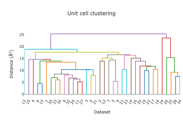
At this point, we can also start looking at the unit cell clustering available in the dials.cosym.html log file. From the dendrogram, it is clear that this does not cleanly split into three groups.

By plotting the value of the unit cell axes (remember, this is a cubic system so a=b=c), the overlap in unit cell dimensions by species is even clearer. While all species seem to have a subtly different unit cell, the natural intra-species variation makes exact separation by unit cell dimension impossible.

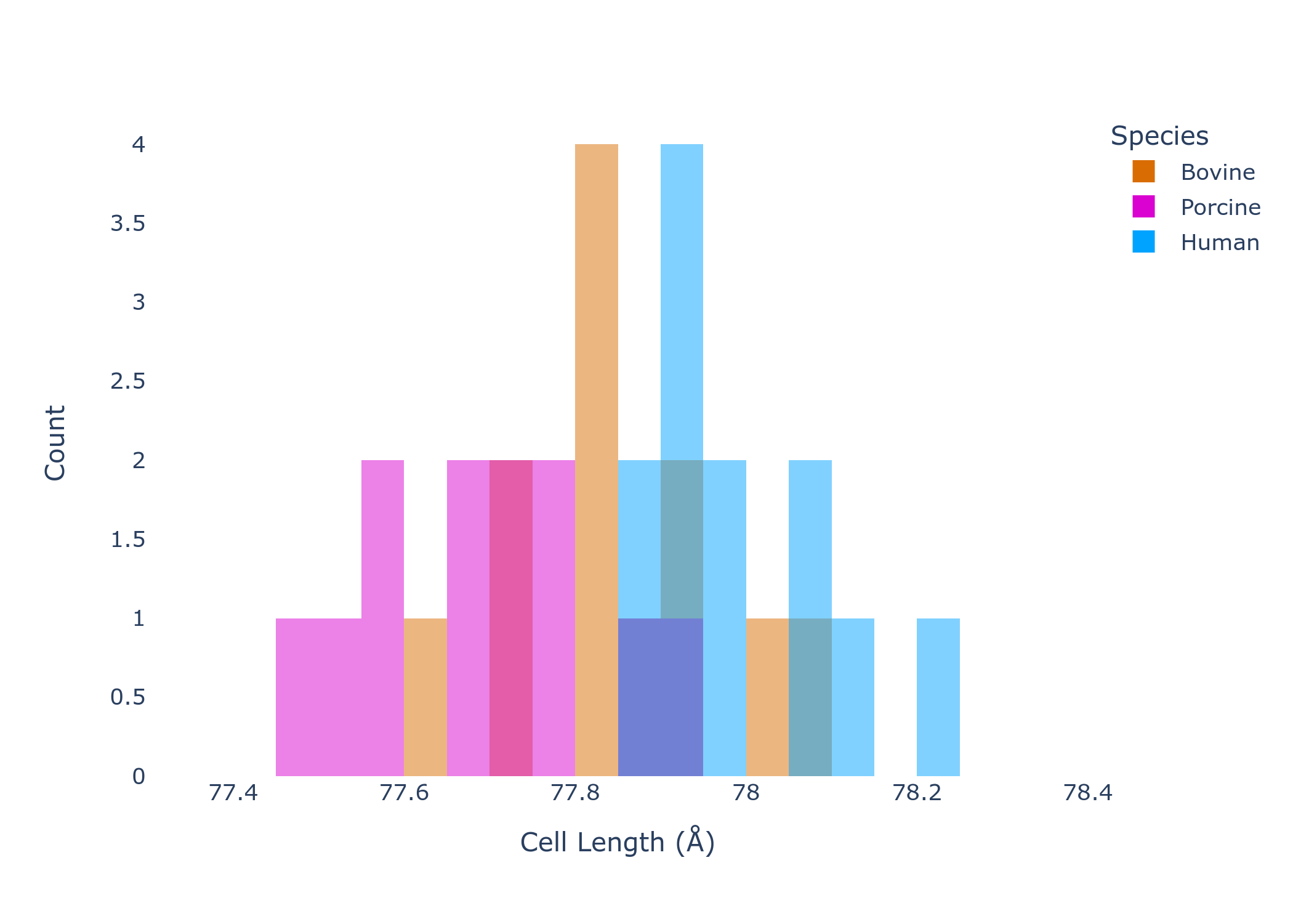
At this point, given no obvious unit cell outliers, the data would be scaled.

dials.scale symmetrized.expt symmetrized.refl

In the output to the terminal you will be able to see the scaling statistics. At a first glance, nothing seems too concerning - the overall CC_1/2 is very close to 1. However, if you open dials.scale.html, you will notice some irregularities. Specifically, the Scale and R_merge vs batch plot seems to indicate the presence of 3 distinct groups.

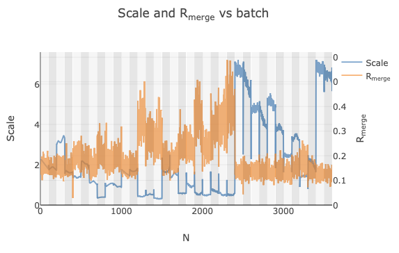
However, these three groups are only obvious because they are grouped by species (an artefact of importing them into DIALS in order). If we did not know which dataset corresponded to each species and all were imported in a random order, this trend would not be so obvious. Instead, some of the datasets may just be discarded as outliers.

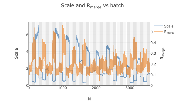
This is where intensity-based clustering is very powerful. We can better see that the differences in scale factor are caused by different groups using dials.correlation_matrix.

dials.correlation_matrix scaled.expt scaled.refl

The commandline output clearly shows the identification of 3 clusters.

Cluster 0
    Number of datasets: 12
    Completeness: 90.2 %
    Multiplicity: 9.55
    Datasets:0,1,2,3,4,5,6,7,8,9,10,11
Cluster 1
    Number of datasets: 12
    Completeness: 90.0 %
    Multiplicity: 9.52
    Datasets:12,13,14,15,16,17,18,19,20,21,22,23
Cluster 2
    Number of datasets: 12
    Completeness: 90.0 %
    Multiplicity: 9.51
    Datasets:24,25,26,27,28,29,30,31,32,33,34,35

We will go through the clustering in the next section. For now, we can output these clusters by re-running the program.

dials.correlation_matrix scaled.expt scaled.refl significant_clusters.output=true

This will give us separated expt/refl files for each cluster. We can then re-scale each individually and merge.

mkdir 0 1 2
cd 0
dials.scale ../cluster_0.expt ../cluster_0.refl
dials.merge scaled.expt scaled.refl
cd ../1
dials.scale ../cluster_1.expt ../cluster_1.refl
dials.merge scaled.expt scaled.refl
cd ../2
dials.scale ../cluster_2.expt ../cluster_2.refl
dials.merge scaled.expt scaled.refl
cd ..

Individually, the scaling statistics look better than the three combined, and we have MTZ files of the separated groups.

Intensity-based Clustering

Now, we will look at the clustering output in more depth to understand how dials.correlation_matrix successfully separated these three sub-groups of 🐮, 🐷, and 💁‍♀️. First, open dials.correlation_matrix.html and click on the Intensity clustering tab. You will then see three more tabs:

Clustering Output Tab	Overview
Hierarchical correlation coefficient clustering	Hierarchical clustering of pairwise CC between all datasets.
Cosym coordinate clustering	Dimension reduction of pairwise CCs and cluster resulting coordinates using OPTICS.
Hierarchical cos angle clustering	Hierarchical clustering of pairwise cosine angles between cosym coordinates.

Intensity-based clustering in DIALS is a multi-step process. For more technical details, see Thompson, A. J. et al. (2025) Acta Cryst. D81, 278-290. The below flowchart summarises the flow of data between the three methods of cluster classification: coordinate, correlation and cosine angle.

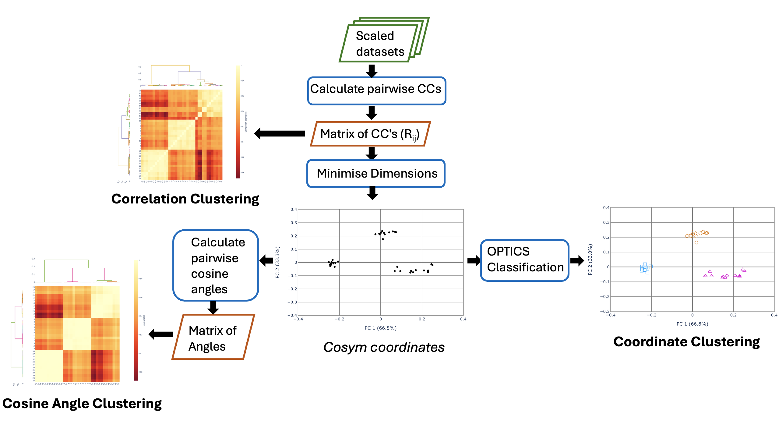
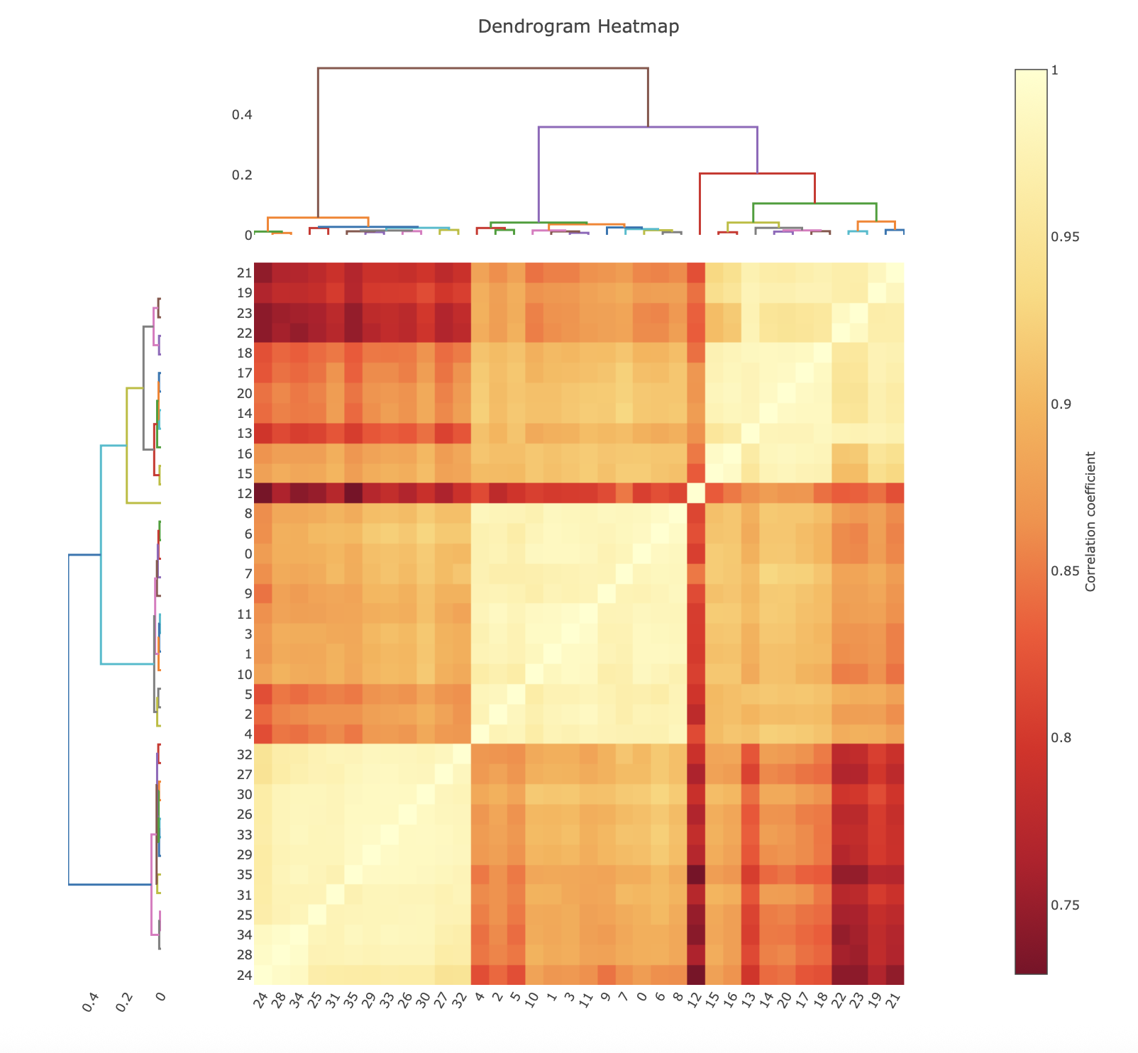
Hierarchical Correlation Coefficient Clustering

The correlation coefficient clustering displays the result of calculating the pairwise correlation coefficients on all datasets. In the heat map, yellow corresponds to a higher correlation, while red is a lower correlation. Note that these colours are relative, with the scale bar showing what the pairwise correlations actually are. The dendrograms on the top and left hand side show how the data clusters, with datasets that join towards the bottom being more similar than groups that join at the top.

Cosym Coordinate Clustering

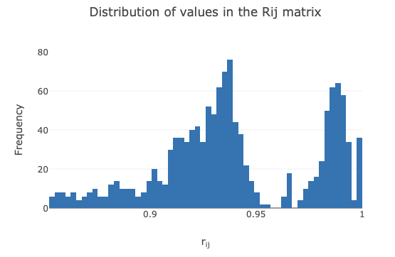
This section describes the coordinate-based clustering approach as well as providing diagnostic graphs for all steps of the algorithm (called cosym as it utilises the same maths as dials.cosym). Within the cosym cluster plots tab, there are four graphs. The first graph displays the pairwise correlation coefficients as a histogram. This can be helpful to visualise if multiple clusters may be present (shown by multiple gaussian-like distributions).

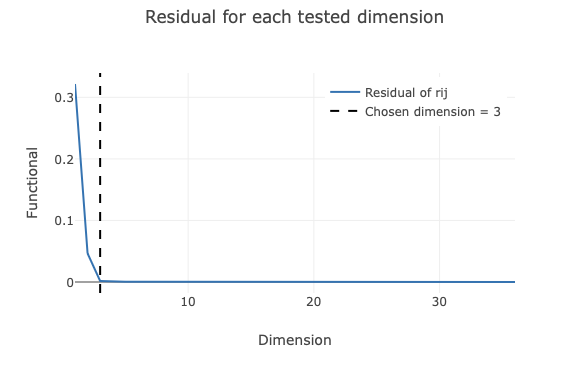
The next plot shows the dimension reduction of the pairwise correlation matrix. The residual (y-axis) of the graph corresponds to the difference between the pairwise correlation matrix and the reduced dimension coordinates. When this value is close to 0, it means that all the information in the high-dimensional correlation matrix is captured by the reduced dimension coordinates. dials.correlation_matrix identifies the elbow point in this plot and defines that as the ideal dimension to use. This dimension reduction is useful, as large datasets quickly become very high dimension. In this example, we have 36 datasets, so the pairwise correlation matrix is 36 x 36, i.e. a 36-dimensional problem. Reducing the dimensions is easier both visually, and computationally. This dimension reduction also has the property of separating random and systematic differences, which can provide useful insight to the data (Diederichs, K. (2017) Acta Cryst. D73, 286-293).

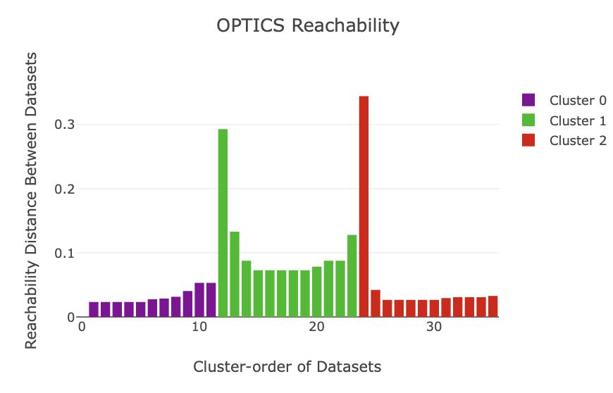
Once the reduced dimension coordinates are optimised, an algorithm called OPTICS is run. Simply, this is an unsupervised machine learning algorithm that looks for dense groups of points in some arbitrary dimensional space. In other words, it looks for dense clusters in our reduced coordinates. OPTICS does this using reachability values (which are plotted). Here, ‘valleys’ correspond to clusters, and ‘spikes’ correspond to boundaries between clusters. Low reachability means datasets are close in space and high reachability means far away in space. This is always based off the preceeding dataset: a high reachability means the previous dataset is far away, which is why clusters often start with a spike in the reachability plot.

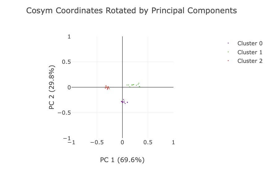
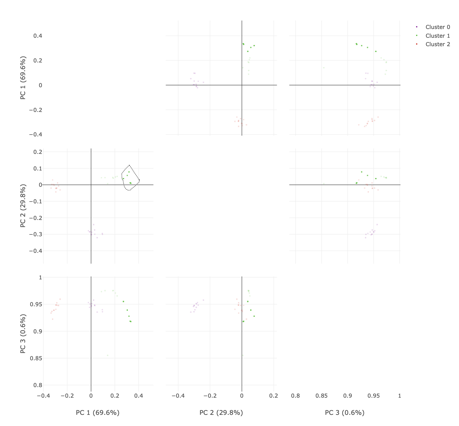
Finally, a plot is given of the reduced dimension coordinates, coloured by the automatic OPTICS classification. Note that only the two most significant dimensions (as identified by principal component analysis) are shown in this plot, and the data are rotated to align with these principal components.

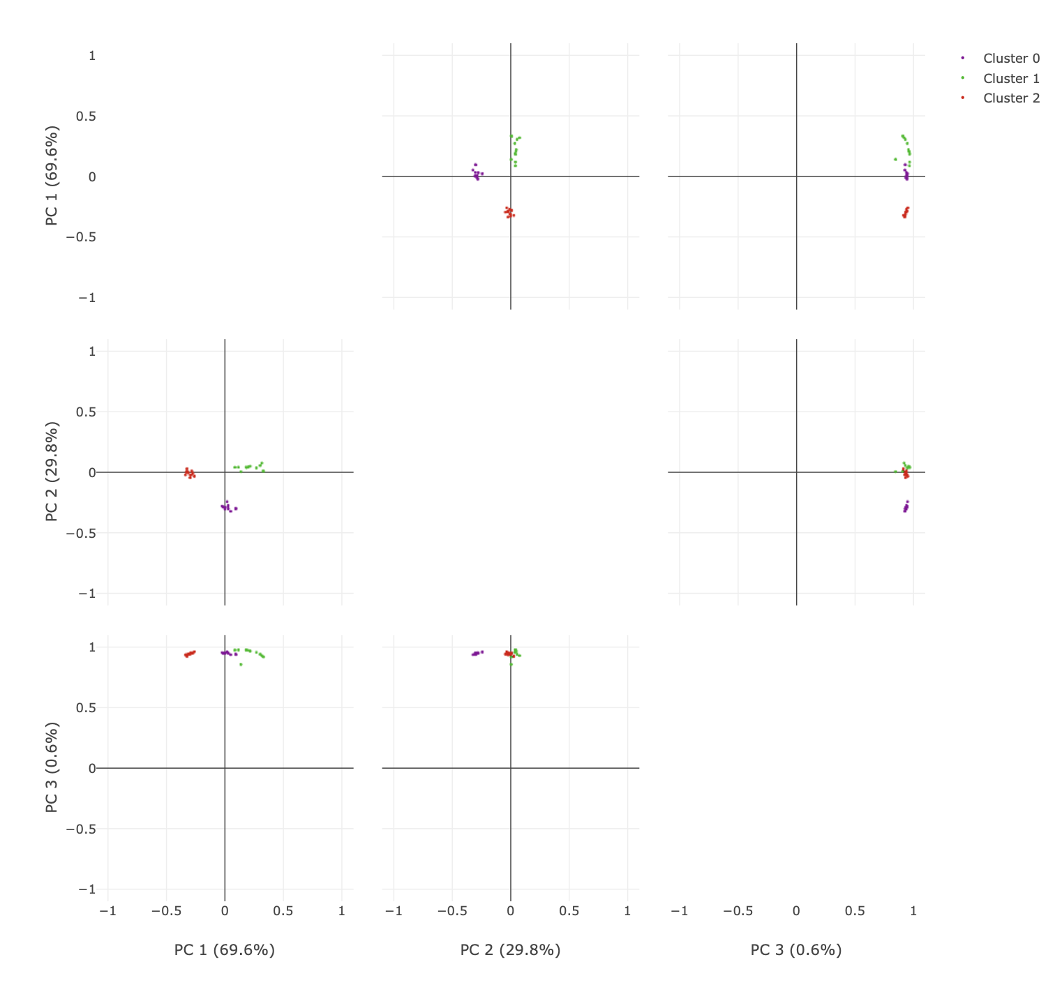
To visualise higher dimensions, go to the principal component analysis tab. Here, the coordinate plot from the previous tab is shown for all combinations of principal components (up to a maximum of 6). There are some neat features here that are useful to explore.

The initial plot is zoomed out.

You can click and drag over the plots to zoom in.

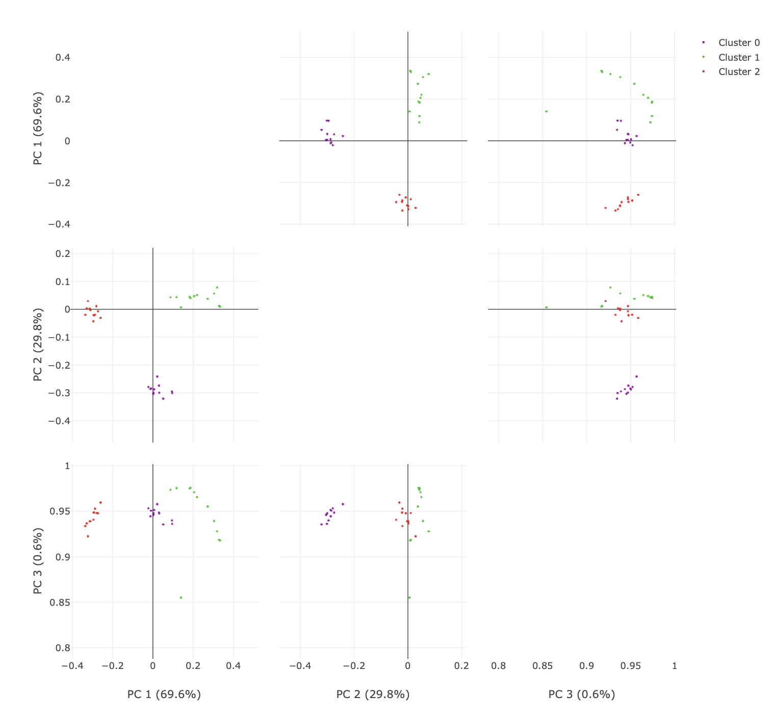
You can also select the lasso tool and highlight only specific data points. The advantage here is being able to easily visualise specific points over multiple dimensions.

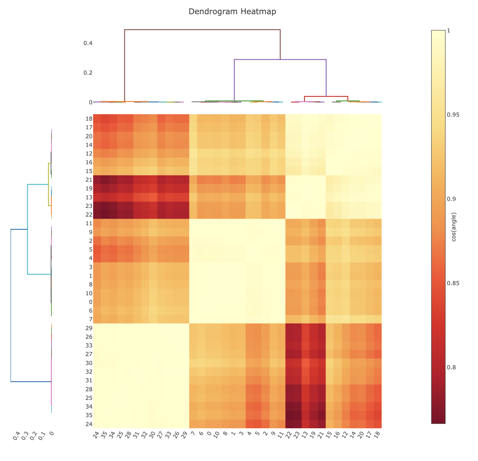
Hierarchical Cos Angle Clustering

Cosine angle clustering is a hierarchical clustering approach similar to correlation coefficient clustering, however the input data are the pairwise angular differences between datasets, after application of the cosym procedure. The minimisation performed during the cosym procedure results in systematic differences being separated in angle (Diederichs, K. (2017) Acta Cryst. D73, 286-293), therefore clustering based on anglular differences will group datasets with low systematic differences. It is presented in an analogous way to the correlation clustering, where the heatmap is representing the cosine of the angular difference.

Automation

All of the intensity-based clustering features in dials.correlation_matrix are also available within xia2.multiplex. xia2.multiplex takes integrated files from multiple crystals, and handles symmetry determination, scaling and filtering in a more automated fashion. It will also scale and merge identified clusters if set up to do so. For more detailed instructions for using the clustering features in xia2.multiplex, see this tutorial. Briefly, the 🐮, 🐷, and 💁‍♀️ from this tutorial can be scaled and merged (with cluster output) using the below command.

mkdir multiplex
cd multiplex
xia2.multiplex ../integrated.expt ../integrated.refl symmetry.space_group=I213 clustering.output_clusters=true clustering.method=coordinate